import yfinance as yf
import matplotlib.pyplot as plt
import numpy as np
import pandas as pd

# Calculate annualized return
def annualized_return(returns, periods_per_year=252):
    compounded_growth = (1 + returns).prod()
    n_periods = returns.count()
    return compounded_growth ** (periods_per_year / n_periods) - 1

# Calculate volatility (annualized standard deviation)
def annualized_volatility(returns, periods_per_year=252):
    return returns.std() * np.sqrt(periods_per_year)

# Calculate Sharpe Ratio
def sharpe_ratio(returns, risk_free_rate=0.02, periods_per_year=252):
    excess_returns = returns - risk_free_rate / periods_per_year
    return np.mean(excess_returns) / np.std(excess_returns) * np.sqrt(periods_per_year)

# Calculate Sortino Ratio
def sortino_ratio(returns, risk_free_rate=0.02, periods_per_year=252):
    downside_returns = returns[returns < 0]
    excess_returns = returns - risk_free_rate / periods_per_year
    return np.mean(excess_returns) / downside_returns.std() * np.sqrt(periods_per_year)

# Maximum drawdown
def max_drawdown(returns):
    cumulative_returns = (1 + returns).cumprod()
    peak = cumulative_returns.expanding(min_periods=1).max()
    drawdown = (cumulative_returns - peak) / peak
return drawdown.min()Mini-Fund Volatility Regime Backtest Analysis (2000–2024)
Abstract
This study evaluates the long-term performance and risk metrics of a high-growth “Mini-Fund” portfolio—consisting of ASML, TSLA, BRK-B, MSFT, ABBV, and LMT—relative to the S&P 500 and Nasdaq-100 benchmarks. Using Hidden Markov Models to categorize market behavior into low, mid, and high volatility regimes, the analysis demonstrates that the optimized “Portfolio-GV-O2” consistently outpaced benchmarks, delivering an annualized return of 30.8% and a Sharpe ratio of 1.25, compared to 11.4% and 0.60 for the S&P 500. The portfolio proved highly resilient during historical recessions, yielding a -2.9% return while the S&P 500 declined by 19.4%. Furthermore, the strategic inclusion of the protective TAIL ETF reduced the maximum drawdown from -35.0% to -27.6%, enhancing downside protection without sacrificing significant growth. CWARP values of 162.3 against the S&P 500 and 78.8 against the Nasdaq-100 further validate the portfolio’s superior risk-adjusted efficiency.
The Philosophy: Investing in Enablers, Not Just Innovators
The concept of a K-wave, named after economist Nikolai Kondratiev, describes long-term economic cycles driven by technological innovation. Each wave—spanning roughly 40-60 years—ushers in transformative advancements, from the Industrial Revolution to the Information Age. We’re now entering what many believe is the sixth K-wave, propelled by AI, clean energy, and advanced manufacturing. While companies at the forefront of these technologies (e.g., pure-play AI startups or speculative renewable energy firms) often dominate headlines, their volatility can make them risky bets for long-term investors
During the 1848 California Gold Rush, it wasn’t the gold miners who reaped the most consistent rewards—it was the “shovelmakers,” the suppliers of tools and infrastructure, who built lasting wealth by enabling the frenzy. Today, as we stand on the cusp of a new technological era defined by artificial intelligence, renewable energy, and advanced manufacturing, a similar strategy can guide us toward sustainable growth.

Instead, our mini-fund targets companies that enable these breakthroughs—those building the “picks and shovels” of the modern era. ASML, for instance, powers the semiconductor industry with its photolithography machines, a cornerstone of AI and computing advancements. Tesla, beyond its electric vehicles, drives innovation in energy storage and autonomous driving infrastructure. Microsoft provides cloud computing and AI platforms that underpin countless applications, while Berkshire Hathaway offers stability and diversified exposure to industrial and financial sectors. AbbVie contributes healthcare innovation, a critical pillar of societal progress, and Lockheed Martin strengthens the portfolio with its leadership in aerospace and defense—sectors poised for growth amid geopolitical shifts and technological integration. This blend of high-growth and value stocks creates a portfolio that captures multiple growth trends while maintaining a solid foundation. By avoiding overexposure to speculative “gold miners,” we aim to deliver consistent returns with reduced downside risk—a strategy validated by our backtest results.
Initial Portfolio Composition
The original portfolio comprises five stocks — ASML Holding N.V. (ASML), SolarEdge Technologies, Inc. (SEDG), Rockwell Automation, Inc. (ROK), Illumina, Inc. (ILMN), and Lockheed Martin Corporation (LMT) — each allocated an equal weight of 20%.
This portfolio was backtested using historical closing prices from January 1, 2000, to January 1, 2024, sourced via Yahoo Finance (yf.download). Daily returns were calculated with pct_change() and cleaned with dropna() to ensure data integrity. The portfolio is benchmarked against the S&P 500 (^GSPC) and Nasdaq-100 (^NDX), reflecting a strategy to measure performance against broad market and technology-focused indices.
This portfolio embodies the “shovelmakers of tomorrow” philosophy outlined earlier. Rather than chasing speculative leaders in emerging technologies, it targets companies that provide critical infrastructure, tools, and services enabling the next Kondratiev wave (K-wave) — such as renewable energy, automation, genomics, and aerospace.
The equal-weight allocation ensures diversification across the following sectors, balancing growth potential with stability:
- Semiconductors
- Solar Energy
- Industrial Automation
- Genomics
- Defense
Companies in the Portfolio
ASML Holding N.V. (ASML)
Sector: Technology (Semiconductors)
Weight: 20%
Role:
ASML is the global leader in photolithography systems, essential for manufacturing integrated circuits (microchips). Its extreme ultraviolet (EUV) lithography machines are critical for producing advanced chips used in AI, 5G, and high-performance computing.
K-Wave Relevance:
ASML is a quintessential shovelmaker, supplying the tools that power the semiconductor industry—a backbone of the sixth K-wave. As demand for AI and IoT grows, ASML’s equipment enables chipmakers like TSMC and Intel to push technological boundaries.
Portfolio Fit:
ASML contributes high-growth potential, capitalizing on secular trends in technology, while its dominant market position adds resilience.
SolarEdge Technologies, Inc. (SEDG)
Sector: Renewable Energy (Solar)
Weight: 20%
Role:
SolarEdge specializes in power optimizers, inverters, and monitoring systems for solar photovoltaic (PV) installations. Its solutions maximize energy efficiency and reliability for residential, commercial, and utility-scale solar projects.
K-Wave Relevance:
The transition to clean energy is a defining feature of the next K-wave, with solar power at the forefront. SolarEdge’s technologies enhance the scalability and affordability of solar energy, positioning it as an enabler of the renewable revolution. Unlike solar panel manufacturers, SolarEdge focuses on the tools that optimize energy output, aligning with the shovelmaker strategy.
Portfolio Fit:
SEDG introduces exposure to the fast-growing renewable energy sector, offering growth potential tempered by the volatility inherent in clean energy markets.
Rockwell Automation, Inc. (ROK)
Sector: Industrials (Automation)
Weight: 20%
Role:
Rockwell Automation provides industrial automation and digital transformation solutions, including programmable logic controllers (PLCs), sensors, and software for smart manufacturing. It serves industries like automotive, food and beverage, and pharmaceuticals.
K-Wave Relevance:
Automation is a cornerstone of the sixth K-wave, driving efficiency in manufacturing and supply chains. Rockwell’s technologies enable “Industry 4.0”—the integration of IoT, AI, and robotics into production—making it a key supplier of tools for industrial innovation. Its focus on software and analytics further aligns with digital transformation trends.
Portfolio Fit:
ROK adds a value-oriented component, balancing growth with stability. Its diversified client base mitigates sector-specific risks, enhancing portfolio resilience.
Illumina, Inc. (ILMN)
Sector: Healthcare (Genomics)
Weight: 20%
Role:
Illumina is a leader in DNA sequencing and genomics, providing instruments, reagents, and software for genetic analysis. Its technologies support applications in personalized medicine, cancer research, and agriculture.
K-Wave Relevance:
Genomics is poised to transform healthcare, a critical pillar of societal progress in the next K-wave. Illumina’s sequencing platforms are the shovels of this revolution, enabling researchers and clinicians to decode genetic data at scale. Its dominance in sequencing technology ensures long-term growth potential.
Portfolio Fit:
ILMN brings exposure to healthcare innovation, a sector with defensive qualities and high growth. It diversifies the portfolio away from pure technology, reducing correlation with market cycles.
Lockheed Martin Corporation (LMT)
Sector: Aerospace and Defense
Weight: 20%
Role:
Lockheed Martin is a global leader in aerospace, defense, and security, known for products like the F-35 fighter jet, missile systems, and space technologies. It serves government and commercial clients worldwide.
K-Wave Relevance:
Defense and aerospace are integral to the next K-wave, driven by geopolitical dynamics and technological advancements (e.g., hypersonics, space exploration). Lockheed Martin’s role as a systems integrator and innovator positions it as an enabler of national security and space infrastructure—a stable shovelmaker in a high-stakes field.
Portfolio Fit:
LMT anchors the portfolio with defensive characteristics, offering steady cash flows and dividends. Its low correlation with tech sectors enhances diversification, mitigating downside risk during market downturns. ownside risk during market downturns.
# Define the stocks and benchmark indices
stocks = ['ASML', 'SEDG', 'ROK', 'ILMN', 'LMT']
benchmark_indices = ['^GSPC', '^NDX']  # S&P 500 and Nasdaq-100

# Download historical data
data = yf.download(stocks + benchmark_indices, start='2000-01-01', end='2024-01-01')['Close']

# Calculate daily returns
returns = data.pct_change()
returns = returns.dropna()

# Equal weights for portfolio
weights = np.array([0.2, 0.2, 0.2, 0.2, 0.2])

# Calculate portfolio returns
portfolio_returns = (returns[stocks] * weights).sum(axis=1)

# Calculate cumulative returns
cumulative_portfolio_returns = (1 + portfolio_returns).cumprod()
cumulative_sp500_returns = (1 + returns['^GSPC']).cumprod()
cumulative_ndx_returns = (1 + returns['^NDX']).cumprod()

# Normalize cumulative returns to 100 for easy comparison
cumulative_portfolio_returns_normalized = cumulative_portfolio_returns / cumulative_portfolio_returns.iloc[0] * 100
cumulative_sp500_returns_normalized = cumulative_sp500_returns / cumulative_sp500_returns.iloc[0] * 100
cumulative_ndx_returns_normalized = cumulative_ndx_returns / cumulative_ndx_returns.iloc[0] * 100


# Plot the data
plt.figure(figsize=(15, 8))

# Plot the portfolio
plt.plot(cumulative_portfolio_returns_normalized, label='Mini-Fund Portfolio', color='blue')

# Plot benchmark indices
plt.plot(cumulative_sp500_returns_normalized, label='S&P 500', linestyle='--', color='orange')
plt.plot(cumulative_ndx_returns_normalized, label='Nasdaq-100', linestyle='--', color='green')

# Add labels and title
plt.title('Growth of Mini-Fund Portfolio vs S&P 500 and Nasdaq-100 (2000-2024)', fontsize=16)
plt.xlabel('Year', fontsize=12)
plt.ylabel('Growth (Normalized to 100)', fontsize=12)
plt.legend(loc='upper left', fontsize=10)

# Show the plot
plt.grid(True)
plt.tight_layout()
plt.show()


# Calculate metrics for mini-fund portfolio
portfolio_metrics = {
    'Annualized Return': annualized_return(portfolio_returns),
    'Volatility': annualized_volatility(portfolio_returns),
    'Sharpe Ratio': sharpe_ratio(portfolio_returns),
    'Sortino Ratio': sortino_ratio(portfolio_returns),
    'Max Drawdown': max_drawdown(portfolio_returns)
}

# Calculate metrics for S&P 500
sp500_metrics = {
    'Annualized Return': annualized_return(returns['^GSPC']),
    'Volatility': annualized_volatility(returns['^GSPC']),
    'Sharpe Ratio': sharpe_ratio(returns['^GSPC']),
    'Sortino Ratio': sortino_ratio(returns['^GSPC']),
    'Max Drawdown': max_drawdown(returns['^GSPC'])
}

# Calculate metrics for Nasdaq-100
ndx_metrics = {
    'Annualized Return': annualized_return(returns['^NDX']),
    'Volatility': annualized_volatility(returns['^NDX']),
    'Sharpe Ratio': sharpe_ratio(returns['^NDX']),
    'Sortino Ratio': sortino_ratio(returns['^NDX']),
    'Max Drawdown': max_drawdown(returns['^NDX'])
}

# Combine results into a DataFrame
metrics_df = pd.DataFrame([portfolio_metrics, sp500_metrics, ndx_metrics], index=['Mini-Fund', 'S&P 500', 'Nasdaq-100'])
pd.set_option('display.width', 1000)
print(metrics_df)
[*********************100%***********************] 7 of 7 completed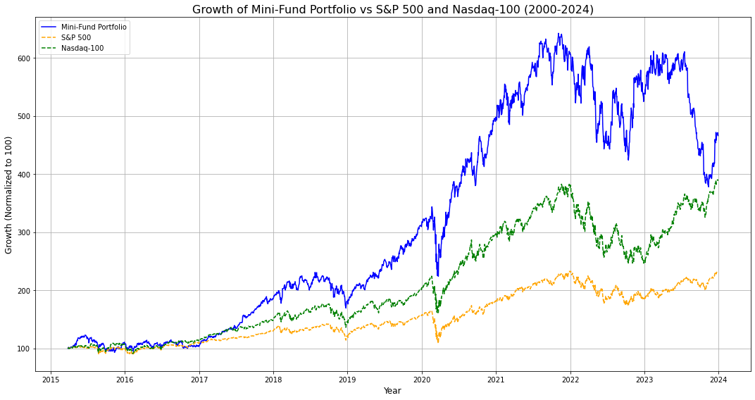
            Annualized Return  Volatility  Sharpe Ratio  Sortino Ratio  Max Drawdown
Mini-Fund            0.194025    0.269933      0.718391       0.997384     -0.411544
S&P 500              0.100897    0.184097      0.506164       0.610701     -0.339250
Nasdaq-100           0.168178    0.225889      0.713269       0.905724     -0.355631
Beginning
import yfinance as yf
import numpy as np
import pandas as pd

# Define the stocks and benchmark indices
stocks = ['ASML', 'NVDA', 'TSLA', 'BRK-B', 'MSFT']
# stocks = ['ASML', 'TSLA', 'BRK-B', 'MSFT']
#stocks = ['ASML', 'TSLA', 'BRK-B', 'MSFT', 'ABBV']
benchmark_indices = ['^GSPC', '^NDX']  # S&P 500 and Nasdaq-100

# Download historical data
data = yf.download(stocks + benchmark_indices, start='2000-01-01', end='2024-01-01')['Close']

# Calculate daily returns
returns = data.pct_change()
returns = returns.dropna()

# Equal weights for portfolio
weights = np.array([0.2, 0.2, 0.2, 0.2, 0.2])
# weights = np.array([0.1639441, 0.2852132, 0.3240187, 0.2268240])
# weights = np.array([0.14, 0.25, 0.29, 0.20, 0.12])

# Calculate portfolio returns
portfolio_returns = (returns[stocks] * weights).sum(axis=1)

# Calculate cumulative returns
cumulative_portfolio_returns = (1 + portfolio_returns).cumprod()
cumulative_sp500_returns = (1 + returns['^GSPC']).cumprod()
cumulative_ndx_returns = (1 + returns['^NDX']).cumprod()


# Calculate metrics for mini-fund portfolio
portfolio_metrics = {
    'Annualized Return': annualized_return(portfolio_returns),
    'Volatility': annualized_volatility(portfolio_returns),
    'Sharpe Ratio': sharpe_ratio(portfolio_returns),
    'Sortino Ratio': sortino_ratio(portfolio_returns),
    'Max Drawdown': max_drawdown(portfolio_returns)
}

# Calculate metrics for S&P 500
sp500_metrics = {
    'Annualized Return': annualized_return(returns['^GSPC']),
    'Volatility': annualized_volatility(returns['^GSPC']),
    'Sharpe Ratio': sharpe_ratio(returns['^GSPC']),
    'Sortino Ratio': sortino_ratio(returns['^GSPC']),
    'Max Drawdown': max_drawdown(returns['^GSPC'])
}

# Calculate metrics for Nasdaq-100
ndx_metrics = {
    'Annualized Return': annualized_return(returns['^NDX']),
    'Volatility': annualized_volatility(returns['^NDX']),
    'Sharpe Ratio': sharpe_ratio(returns['^NDX']),
    'Sortino Ratio': sortino_ratio(returns['^NDX']),
    'Max Drawdown': max_drawdown(returns['^NDX'])
}

# Normalize cumulative returns to 100 for easy comparison
cumulative_portfolio_returns_normalized = cumulative_portfolio_returns / cumulative_portfolio_returns.iloc[0] * 100
cumulative_sp500_returns_normalized = cumulative_sp500_returns / cumulative_sp500_returns.iloc[0] * 100
cumulative_ndx_returns_normalized = cumulative_ndx_returns / cumulative_ndx_returns.iloc[0] * 100

# Plot the data
plt.figure(figsize=(15, 8))

# Plot the portfolio
plt.plot(cumulative_portfolio_returns_normalized, label='Portfolio-GV', color='blue')

# Plot benchmark indices
plt.plot(cumulative_sp500_returns_normalized, label='S&P 500', linestyle='--', color='orange')
plt.plot(cumulative_ndx_returns_normalized, label='Nasdaq-100', linestyle='--', color='green')

# Add labels and title
plt.title('Growth of Portfolio-GV vs S&P 500 and Nasdaq-100 (2000-2024)', fontsize=16)
plt.xlabel('Year', fontsize=12)
plt.ylabel('Growth (Normalized to 100)', fontsize=12)
plt.legend(loc='upper left', fontsize=10)

# Show the plot
plt.grid(True)
plt.tight_layout()
plt.show()

# Combine results into a DataFrame
metrics_df = pd.DataFrame([portfolio_metrics, sp500_metrics, ndx_metrics], index=['Mini-Fund', 'S&P 500', 'Nasdaq-100'])
print(metrics_df)
[*********************100%***********************] 7 of 7 completed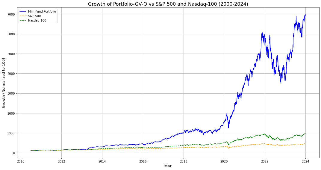
            Annualized Return  Volatility  Sharpe Ratio  Sortino Ratio  Max Drawdown
Mini-Fund            0.367925    0.272138      1.214923       1.683422     -0.421506
S&P 500              0.119445    0.174019      0.621038       0.762031     -0.339250
Nasdaq-100           0.181999    0.207497      0.813858       1.043914     -0.355631
import yfinance as yf
import numpy as np
import pandas as pd
# Define the stocks and benchmark indices
# stocks = ['ASML', 'NVDA', 'TSLA', 'BRK-B', 'MSFT']
stocks = ['ASML', 'TSLA', 'BRK-B', 'MSFT']
# stocks = ['ASML', 'TSLA', 'BRK-B', 'MSFT', 'ABBV']
benchmark_indices = ['^GSPC', '^NDX'] # S&P 500 and Nasdaq-100
# Download historical data
data = yf.download(stocks + benchmark_indices, start='2000-01-01', end='2024-01-01')['Adj Close']
# Calculate daily returns
returns = data.pct_change()
returns = returns.dropna()
# Equal weights for portfolio
weights = np.array([0.2, 0.2, 0.2, 0.2, 0.2, 0.2])
# weights = np.array([0.1639441, 0.2852132, 0.3240187, 0.2268240])
# weights = np.array([0.14, 0.25, 0.29, 0.20, 0.12])
# Calculate portfolio returns
portfolio_returns = (returns[stocks] * weights).sum(axis=1)
# Calculate cumulative returns
cumulative_portfolio_returns = (1 + portfolio_returns).cumprod()
cumulative_sp500_returns = (1 + returns['^GSPC']).cumprod()
cumulative_ndx_returns = (1 + returns['^NDX']).cumprod()
# Calculate metrics for mini-fund portfolio
portfolio_metrics = {
'Annualized Return': annualized_return(portfolio_returns),
'Volatility': annualized_volatility(portfolio_returns),
'Sharpe Ratio': sharpe_ratio(portfolio_returns),
'Sortino Ratio': sortino_ratio(portfolio_returns),
'Max Drawdown': max_drawdown(portfolio_returns)
}
# Calculate metrics for S&P 500
sp500_metrics = {
'Annualized Return': annualized_return(returns['^GSPC']),
'Volatility': annualized_volatility(returns['^GSPC']),
'Sharpe Ratio': sharpe_ratio(returns['^GSPC']),
'Sortino Ratio': sortino_ratio(returns['^GSPC']),
'Max Drawdown': max_drawdown(returns['^GSPC'])
}
# Calculate metrics for Nasdaq-100
ndx_metrics = {
'Annualized Return': annualized_return(returns['^NDX']),
'Volatility': annualized_volatility(returns['^NDX']),
'Sharpe Ratio': sharpe_ratio(returns['^NDX']),
'Sortino Ratio': sortino_ratio(returns['^NDX']),
'Max Drawdown': max_drawdown(returns['^NDX'])
}
# Normalize cumulative returns to 100 for easy comparison
cumulative_portfolio_returns_normalized = cumulative_portfolio_returns / cumulative_portfolio_returns.iloc[0] * 100
cumulative_sp500_returns_normalized = cumulative_sp500_returns / cumulative_sp500_returns.iloc[0] * 100
cumulative_ndx_returns_normalized = cumulative_ndx_returns / cumulative_ndx_returns.iloc[0] * 100
# Plot the data
plt.figure(figsize=(15, 8))
# Plot the portfolio
plt.plot(cumulative_portfolio_returns_normalized, label='Mini-Fund Portfolio', color='blue')
# Plot benchmark indices
plt.plot(cumulative_sp500_returns_normalized, label='S&P 500', linestyle='--', color='orange')
plt.plot(cumulative_ndx_returns_normalized, label='Nasdaq-100', linestyle='--', color='green')
# Add labels and title
plt.title('Growth of Portfolio-GV-O1 vs S&P 500 and Nasdaq-100 (2000-2024)', fontsize=16)
plt.xlabel('Year', fontsize=12)
plt.ylabel('Growth (Normalized to 100)', fontsize=12)
plt.legend(loc='upper left', fontsize=10)
# Show the plot
plt.grid(True)
plt.tight_layout()
plt.show()
# Combine results into a DataFrame
metrics_df = pd.DataFrame([portfolio_metrics, sp500_metrics, ndx_metrics], index=['Mini-Fund', 'S&P 500', 'Nasdaq-100'])
print(metrics_df)[*********************100%***********************] 7 of 7 completed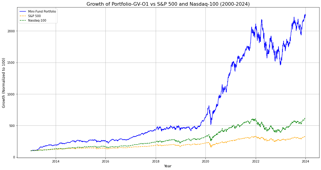
            Annualized Return  Volatility  Sharpe Ratio  Sortino Ratio  Max Drawdown
Mini-Fund            0.325947    0.240479      1.211467       1.630888     -0.371925
S&P 500              0.113679    0.172243      0.595699       0.721428     -0.339250
Nasdaq-100           0.179487    0.210365      0.795558       1.003233     -0.355631
import yfinance as yf
import numpy as np
import pandas as pd
# Define the stocks and benchmark indices
#stocks = ['ASML', 'NVDA', 'TSLA', 'BRK-B', 'MSFT']
#stocks = ['ASML', 'TSLA', 'BRK-B', 'MSFT']
stocks = ['ASML', 'TSLA', 'BRK-B', 'MSFT', 'ABBV', 'LMT']
benchmark_indices = ['^GSPC', '^NDX'] # S&P 500 and Nasdaq-100
# Download historical data
data = yf.download(stocks + benchmark_indices, start='2000-01-01', end='2024-01-01')['Adj Close']
# Calculate daily returns
returns = data.pct_change()
returns = returns.dropna()
# Equal weights for portfolio
# weights = np.array([0.2, 0.2, 0.2, 0.2, 0.2])
# weights = np.array([0.1639441, 0.2852132, 0.3240187, 0.2268240])
weights = np.array([0.15, 0.20, 0.25, 0.18, 0.10, 0.12])
# Calculate portfolio returns
portfolio_returns = (returns[stocks] * weights).sum(axis=1)
# Calculate cumulative returns
cumulative_portfolio_returns = (1 + portfolio_returns).cumprod()
cumulative_sp500_returns = (1 + returns['^GSPC']).cumprod()
cumulative_ndx_returns = (1 + returns['^NDX']).cumprod()
# Calculate metrics for mini-fund portfolio
portfolio_metrics = {
'Annualized Return': annualized_return(portfolio_returns),
'Volatility': annualized_volatility(portfolio_returns),
'Sharpe Ratio': sharpe_ratio(portfolio_returns),
'Sortino Ratio': sortino_ratio(portfolio_returns),
'Max Drawdown': max_drawdown(portfolio_returns)
}
# Calculate metrics for S&P 500
sp500_metrics = {
'Annualized Return': annualized_return(returns['^GSPC']),
'Volatility': annualized_volatility(returns['^GSPC']),
'Sharpe Ratio': sharpe_ratio(returns['^GSPC']),
'Sortino Ratio': sortino_ratio(returns['^GSPC']),
'Max Drawdown': max_drawdown(returns['^GSPC'])
}
# Calculate metrics for Nasdaq-100
ndx_metrics = {
'Annualized Return': annualized_return(returns['^NDX']),
'Volatility': annualized_volatility(returns['^NDX']),
'Sharpe Ratio': sharpe_ratio(returns['^NDX']),
'Sortino Ratio': sortino_ratio(returns['^NDX']),
'Max Drawdown': max_drawdown(returns['^NDX'])
}
# Normalize cumulative returns to 100 for easy comparison
cumulative_portfolio_returns_normalized = cumulative_portfolio_returns / cumulative_portfolio_returns.iloc[0] * 100
cumulative_sp500_returns_normalized = cumulative_sp500_returns / cumulative_sp500_returns.iloc[0] * 100
cumulative_ndx_returns_normalized = cumulative_ndx_returns / cumulative_ndx_returns.iloc[0] * 100
# Plot the data
plt.figure(figsize=(15, 8))
# Plot the portfolio
plt.plot(cumulative_portfolio_returns_normalized, label='Mini-Fund Portfolio', color='blue')
# Plot benchmark indices
plt.plot(cumulative_sp500_returns_normalized, label='S&P 500', linestyle='--', color='orange')
plt.plot(cumulative_ndx_returns_normalized, label='Nasdaq-100', linestyle='--', color='green')
# Add labels and title
plt.title('Growth of Portfolio-GV-O2 vs S&P 500 and Nasdaq-100 (2000-2024)', fontsize=16)
plt.xlabel('Year', fontsize=12)
plt.ylabel('Growth (Normalized to 100)', fontsize=12)
plt.legend(loc='upper left', fontsize=10)
# Show the plot
plt.grid(True)
plt.tight_layout()
plt.show()
# Combine results into a DataFrame
metrics_df = pd.DataFrame([portfolio_metrics, sp500_metrics, ndx_metrics], index=['Mini-Fund', 'S&P 500', 'Nasdaq-100'])
print(metrics_df)[*********************100%***********************] 8 of 8 completed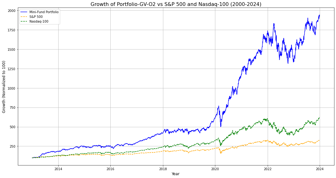
            Annualized Return  Volatility  Sharpe Ratio  Sortino Ratio  Max Drawdown
Mini-Fund            0.308158    0.218942      1.246309       1.642653     -0.350050
S&P 500              0.113679    0.172243      0.595699       0.721428     -0.339250
Nasdaq-100           0.179487    0.210365      0.795558       1.003233     -0.355631
import yfinance as yf
import numpy as np
import pandas as pd
import matplotlib.pyplot as plt
import seaborn as sns
# Define the stocks and benchmark indices
stocks = ['ASML', 'TSLA', 'BRK-B', 'MSFT', 'ABBV', 'LMT']
benchmark_indices = ['^GSPC', '^NDX'] # S&P 500 and Nasdaq-100
# Download historical data
data = yf.download(stocks + benchmark_indices, start='2000-01-01', end='2024-01-01')['Adj Close']
# Calculate daily returns
returns = data.pct_change().dropna()
# Equal weights for portfolio
weights = np.array([0.15, 0.20, 0.25, 0.18, 0.10, 0.12])
# Calculate portfolio returns
portfolio_returns = (returns[stocks] * weights).sum(axis=1)
# Plot the density plots for Portfolio, S&P 500, and Nasdaq-100 returns
plt.figure(figsize=(15, 8))
# Full Density Plot
sns.kdeplot(portfolio_returns, label='Portfolio-GV-O2', color='blue', shade=True, clip=(-0.06, 0.06))
sns.kdeplot(returns['^GSPC'], label='S&P 500', color='orange', shade=True, clip=(-0.06, 0.06))
sns.kdeplot(returns['^NDX'], label='Nasdaq-100', color='green', shade=True, clip=(-0.06, 0.06))
plt.title('Zoomed-In Density Plot: Left and Right Tails', fontsize=16)
plt.xlabel('Daily Return', fontsize=12)
plt.ylabel('Density', fontsize=12)
plt.legend(loc='upper right', fontsize=10)
# Adjust layout and show plot
plt.tight_layout()
plt.grid(True)
plt.show()[*********************100%***********************] 8 of 8 completed
<ipython-input-23-b30301a8e790>:28: FutureWarning:
`shade` is now deprecated in favor of `fill`; setting `fill=True`.
This will become an error in seaborn v0.14.0; please update your code.
sns.kdeplot(portfolio_returns, label='Mini-Fund Portfolio', color='blue', shade=True, clip=(-0.06, 0.06))
<ipython-input-23-b30301a8e790>:29: FutureWarning:
`shade` is now deprecated in favor of `fill`; setting `fill=True`.
This will become an error in seaborn v0.14.0; please update your code.
sns.kdeplot(returns['^GSPC'], label='S&P 500', color='orange', shade=True, clip=(-0.06, 0.06))
<ipython-input-23-b30301a8e790>:30: FutureWarning:
`shade` is now deprecated in favor of `fill`; setting `fill=True`.
This will become an error in seaborn v0.14.0; please update your code.
sns.kdeplot(returns['^NDX'], label='Nasdaq-100', color='green', shade=True, clip=(-0.06, 0.06))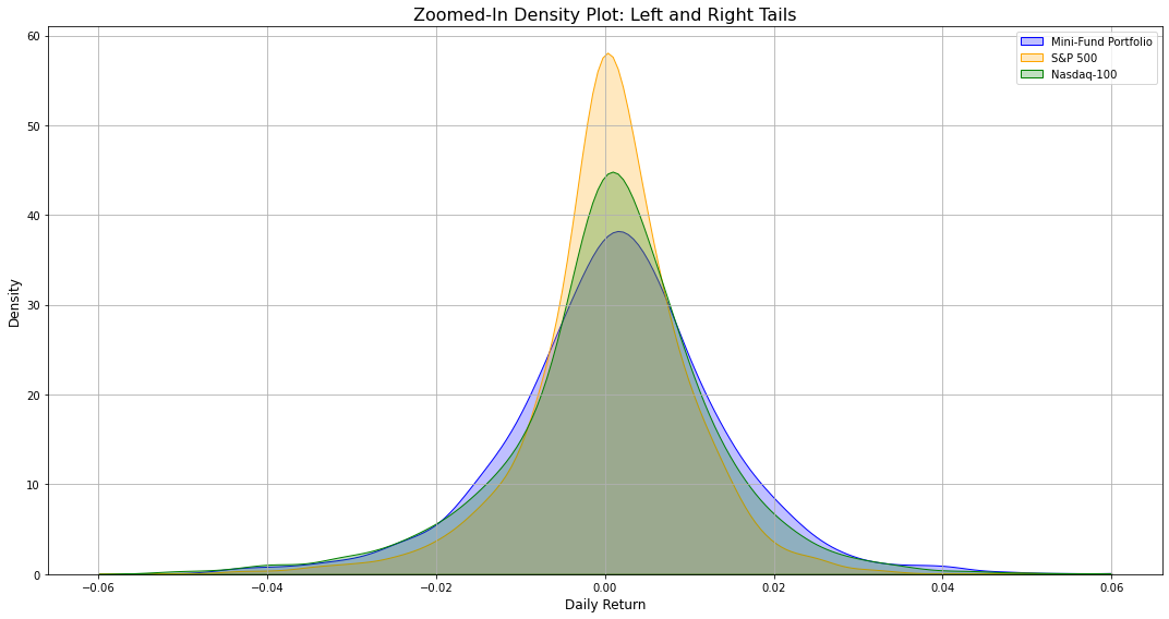
Perf across vol regimes
import yfinance as yf
import numpy as np
import pandas as pd
import matplotlib.pyplot as plt
from hmmlearn.hmm import GaussianHMM

# Define the stocks and benchmark indices
stocks = ['ASML', 'TSLA', 'BRK-B', 'MSFT', 'ABBV', 'LMT']
benchmark_indices = ['^GSPC', '^NDX']  # S&P 500 and Nasdaq-100

# Download historical data
data = yf.download(stocks + benchmark_indices, start='2000-01-01', end='2024-01-01')['Adj Close']

# Calculate daily returns
returns = data.pct_change().dropna()

# Equal weights for portfolio
weights = np.array([0.15, 0.20, 0.25, 0.18, 0.10, 0.12])

# Calculate portfolio returns
portfolio_returns = (returns[stocks] * weights).sum(axis=1)

# Fit a 3-state HMM to detect volatility regimes
model = GaussianHMM(n_components=3, covariance_type="full", n_iter=1000)
model.fit(portfolio_returns.values.reshape(-1, 1))

# Predict regimes
hidden_states = model.predict(portfolio_returns.values.reshape(-1, 1))

# Add hidden state labels to returns DataFrame
returns_df = pd.DataFrame({
    'Portfolio Returns': portfolio_returns,
    '^GSPC Returns': returns['^GSPC'],
    '^NDX Returns': returns['^NDX'],
    'Hidden State': hidden_states
})

# Calculate average volatility of each regime to determine regime labels
average_volatility = returns_df.groupby('Hidden State')['Portfolio Returns'].std()

# Sort the volatilities to label regimes
volatility_rank = average_volatility.sort_values().index
regime_labels = {volatility_rank[0]: 'Low Volatility',
                 volatility_rank[1]: 'Mid Volatility',
                 volatility_rank[2]: 'High Volatility'}

# Add regime labels to DataFrame
returns_df['Volatility Regime'] = returns_df['Hidden State'].map(regime_labels)

# Define metric functions
def annualized_return(returns, periods_per_year=252):
    compounded_growth = (1 + returns).prod()
    n_periods = returns.count()
    return compounded_growth ** (periods_per_year / n_periods) - 1

def annualized_volatility(returns, periods_per_year=252):
    return returns.std() * np.sqrt(periods_per_year)

def sharpe_ratio(returns, risk_free_rate=0.02, periods_per_year=252):
    excess_returns = returns - risk_free_rate / periods_per_year
    return np.mean(excess_returns) / np.std(excess_returns) * np.sqrt(periods_per_year)

def sortino_ratio(returns, risk_free_rate=0.02, periods_per_year=252):
    downside_returns = returns[returns < 0]
    excess_returns = returns - risk_free_rate / periods_per_year
    return np.mean(excess_returns) / downside_returns.std() * np.sqrt(periods_per_year)

def max_drawdown(returns):
    cumulative_returns = (1 + returns).cumprod()
    peak = cumulative_returns.expanding(min_periods=1).max()
    drawdown = (cumulative_returns - peak) / peak
    return drawdown.min()

# Calculate metrics for each volatility regime for portfolio, S&P 500, and Nasdaq-100
metrics = {}

for regime in ['Low Volatility', 'Mid Volatility', 'High Volatility']:
    state_data = returns_df[returns_df['Volatility Regime'] == regime]
    state_metrics = {}

    for col in ['Portfolio Returns', '^GSPC Returns', '^NDX Returns']:
        state_metrics[col] = {
            'Annualized Return': annualized_return(state_data[col]),
            'Volatility': annualized_volatility(state_data[col]),
            'Sharpe Ratio': sharpe_ratio(state_data[col]),
            'Sortino Ratio': sortino_ratio(state_data[col]),
            'Max Drawdown': max_drawdown(state_data[col])
        }

    metrics[regime] = state_metrics

# Convert metrics to a DataFrame for better visualization
metrics_dict = {}
for regime, data in metrics.items():
    for asset, values in data.items():
        row_key = f"{regime} - {asset.replace('Portfolio Returns', 'Mini-Fund').replace('^GSPC Returns', 'S&P 500').replace('^NDX Returns', 'Nasdaq-100')}"
        metrics_dict[row_key] = values

metrics_df = pd.DataFrame(metrics_dict).T
metrics_df = metrics_df.rename_axis('Regime and Asset').reset_index()

# Group the table display by Low/Mid/High Volatility Regimes to enhance readability
grouped_metrics = metrics_df.copy()

# Formatting the DataFrame to show Regime and Metrics without repetition of the regime
grouped_metrics['Volatility Regime'] = grouped_metrics['Regime and Asset'].str.extract(r'^(Low|Mid|High) Volatility')
grouped_metrics['Asset'] = grouped_metrics['Regime and Asset'].str.replace(r'^(Low|Mid|High) Volatility - ', '')
grouped_metrics.drop(columns=['Regime and Asset'], inplace=True)

# Reorder columns for better readability
grouped_metrics = grouped_metrics[['Volatility Regime', 'Asset', 'Annualized Return', 'Volatility', 'Sharpe Ratio', 'Sortino Ratio', 'Max Drawdown']]

# Sorting the DataFrame by 'Volatility Regime' to ensure grouping
grouped_metrics = grouped_metrics.sort_values(by=['Volatility Regime', 'Asset']).reset_index(drop=True)

# Display in a more readable format
pd.set_option('display.max_columns', None)
pd.set_option('display.float_format', '{:.4f}'.format)
pd.set_option('display.width', 1000)
print("\nPerformance Metrics Grouped by Volatility Regime:")
print(grouped_metrics)

# Plotting cumulative returns for each regime
plt.figure(figsize=(15, 8))

for regime in ['Low Volatility', 'Mid Volatility', 'High Volatility']:
    state_data = returns_df[returns_df['Volatility Regime'] == regime]
    cumulative_portfolio_returns = (1 + state_data['Portfolio Returns']).cumprod()
    cumulative_sp500_returns = (1 + state_data['^GSPC Returns']).cumprod()
    cumulative_ndx_returns = (1 + state_data['^NDX Returns']).cumprod()

    plt.plot(cumulative_portfolio_returns, label=f'{regime} - Mini-Fund Cumulative Returns', linestyle='-', color=f'C{list(regime_labels.values()).index(regime)}')
    plt.plot(cumulative_sp500_returns, label=f'{regime} - S&P 500 Cumulative Returns', linestyle='--', color=f'C{list(regime_labels.values()).index(regime)}')
    plt.plot(cumulative_ndx_returns, label=f'{regime} - Nasdaq-100 Cumulative Returns', linestyle=':', color=f'C{list(regime_labels.values()).index(regime)}')

# Add labels and title
plt.title('Cumulative Returns of Portfolio-GV-O2, S&P 500, and Nasdaq-100 Across Volatility Regimes', fontsize=16)
plt.xlabel('Date', fontsize=12)
plt.ylabel('Cumulative Growth', fontsize=12)
plt.legend(loc='upper left', fontsize=10)

# Show the plot
plt.grid(True)
plt.tight_layout()
plt.show()
[*********************100%***********************] 8 of 8 completed
Model is not converging. Current: 8306.194727967259 is not greater than 8306.204205929746. Delta is -0.009477962486926117
Performance Metrics Grouped by Volatility Regime:
  Volatility Regime                         Asset  Annualized Return  Volatility  Sharpe Ratio  Sortino Ratio  Max Drawdown
0              High   High Volatility - Mini-Fund            -0.8314      0.8617       -1.6850        -2.4929       -0.3083
1              High  High Volatility - Nasdaq-100            -0.7188      0.8288       -1.1669        -2.0536       -0.2297
2              High     High Volatility - S&P 500            -0.8402      0.8390       -1.8236        -3.2338       -0.3064
3               Low    Low Volatility - Mini-Fund             0.3906      0.1553        2.0735         3.2254       -0.1154
4               Low   Low Volatility - Nasdaq-100             0.3058      0.1421        1.8093         2.5148       -0.1106
5               Low      Low Volatility - S&P 500             0.2072      0.1101        1.5845         2.1873       -0.1028
6               Mid    Mid Volatility - Mini-Fund             0.1974      0.2961        0.6896         1.0894       -0.3166
7               Mid   Mid Volatility - Nasdaq-100            -0.0683      0.2950       -0.1602        -0.2455       -0.4023
8               Mid      Mid Volatility - S&P 500            -0.0423      0.2274       -0.1644        -0.2437       -0.3408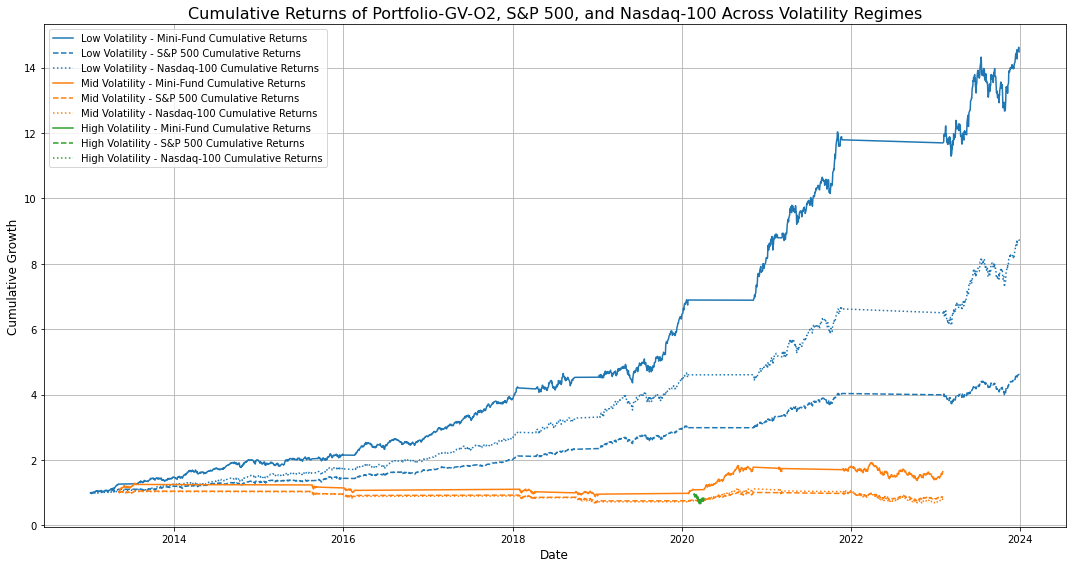
import yfinance as yf
import numpy as np
import pandas as pd
import matplotlib.pyplot as plt
import seaborn as sns
from hmmlearn.hmm import GaussianHMM

# Define the stocks and benchmark indices
stocks = ['ASML', 'TSLA', 'BRK-B', 'MSFT', 'ABBV', 'LMT']
benchmark_indices = ['^GSPC', '^NDX']  # S&P 500 and Nasdaq-100

# Download historical data
data = yf.download(stocks + benchmark_indices, start='2000-01-01', end='2024-01-01')['Adj Close']

# Calculate daily returns
returns = data.pct_change().dropna()

# Equal weights for portfolio
weights = np.array([0.15, 0.20, 0.25, 0.18, 0.10, 0.12])

# Calculate portfolio returns
portfolio_returns = (returns[stocks] * weights).sum(axis=1)

# Fit a 3-state HMM to detect volatility regimes
model = GaussianHMM(n_components=3, covariance_type="full", n_iter=1000)
model.fit(portfolio_returns.values.reshape(-1, 1))

# Predict regimes
hidden_states = model.predict(portfolio_returns.values.reshape(-1, 1))

# Add hidden state labels to returns DataFrame
returns_df = pd.DataFrame({
    'Date': returns.index,
    'Portfolio Returns': portfolio_returns,
    'S&P 500 Returns': returns['^GSPC'],
    'Nasdaq-100 Returns': returns['^NDX'],
    'Hidden State': hidden_states
})

# Calculate average volatility of each regime to determine regime labels
average_volatility = returns_df.groupby('Hidden State')['Portfolio Returns'].std()

# Sort the volatilities to label regimes
volatility_rank = average_volatility.sort_values().index
regime_labels = {volatility_rank[0]: 'Low Volatility',
                 volatility_rank[1]: 'Mid Volatility',
                 volatility_rank[2]: 'High Volatility'}

# Add regime labels to DataFrame
returns_df['Volatility Regime'] = returns_df['Hidden State'].map(regime_labels)

# Calculate cumulative returns for each asset and add to DataFrame
returns_df['Cumulative Portfolio Returns'] = (1 + returns_df['Portfolio Returns']).cumprod()
returns_df['Cumulative S&P 500 Returns'] = (1 + returns_df['S&P 500 Returns']).cumprod()
returns_df['Cumulative Nasdaq-100 Returns'] = (1 + returns_df['Nasdaq-100 Returns']).cumprod()

# Melt the DataFrame for seaborn compatibility
cumulative_returns_df = pd.melt(
    returns_df,
    id_vars=['Date', 'Volatility Regime'],
    value_vars=['Cumulative Portfolio Returns', 'Cumulative S&P 500 Returns', 'Cumulative Nasdaq-100 Returns'],
    var_name='Asset',
    value_name='Cumulative Returns'
)

# Create a faceted plot using seaborn's FacetGrid
g = sns.FacetGrid(cumulative_returns_df, col='Volatility Regime', hue='Asset', col_wrap=3, height=4, aspect=1.5)
g.map(plt.plot, 'Date', 'Cumulative Returns').add_legend()

# Adjust plot aesthetics
g.set_axis_labels('Date', 'Cumulative Growth')
g.set_titles(col_template='{col_name} Regime')
g.fig.suptitle('Cumulative Returns Across Volatility Regimes for Portfolio, S&P 500, and Nasdaq-100', y=1.05)

plt.tight_layout()
plt.show()
[*********************100%***********************] 8 of 8 completed
Model is not converging. Current: 8305.528897318622 is not greater than 8305.57159532981. Delta is -0.042698011187894735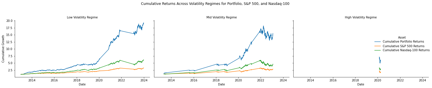
import yfinance as yf
import numpy as np
import pandas as pd
import matplotlib.pyplot as plt
from scipy.stats import norm
from tabulate import tabulate

from scipy.stats import t
from arch import arch_model  # To use GARCH for volatility forecasting

# Define risk-free rate (approximation)
risk_free_rate = 0.02  # 2% annually

# Define the stocks and benchmark indices
stocks = ['ASML', 'TSLA', 'BRK-B', 'MSFT', 'ABBV', 'LMT']  # Example portfolio stocks
benchmark_indices = ['^GSPC', '^NDX']  # S&P 500 and Nasdaq-100

# Download historical data
data = yf.download(stocks + benchmark_indices, start='2000-01-01', end='2024-01-01')['Adj Close']

# Calculate daily returns
returns = data.pct_change().dropna()

# Equal weights for portfolio
weights = np.array([0.15, 0.20, 0.25, 0.18, 0.10, 0.12])

# Calculate portfolio returns
portfolio_returns = (returns[stocks] * weights).sum(axis=1)

# Calculate benchmark returns
market_returns = returns['^GSPC']  # S&P 500 as benchmark

# Alpha, Beta, R-Square
cov_matrix = np.cov(portfolio_returns, market_returns)
beta_portfolio = cov_matrix[0, 1] / cov_matrix[1, 1]
alpha_portfolio = np.mean(portfolio_returns) - beta_portfolio * np.mean(market_returns)
r_square = 1 - (np.var(portfolio_returns - beta_portfolio * market_returns) / np.var(portfolio_returns))

# Value at Risk (VaR) and Expected Shortfall (ES)
import numpy as np
from scipy.stats import norm

def var_es(returns, confidence_level=0.95):
    """
    Calculate VaR and Expected Shortfall using the normal distribution.

    Args:
        returns (pd.Series): A pandas Series of historical returns.
        confidence_level (float): Confidence level for VaR and ES calculation.

    Returns:
        Tuple: VaR and ES for 1-month, 6-month, and 1-year periods.
    """
    # Calculate the mean return and standard deviation (daily)
    mean_return_daily = returns.mean()
    std_dev_daily = returns.std()

    # z-score for the given confidence level (left tail)
    z = norm.ppf(confidence_level)

    # Time horizons in days
    periods = {'1m': 21, '6m': 126, '1y': 252}

    var_list = []
    es_list = []

    for days in periods.values():
        mean_return_period = mean_return_daily * days
        std_dev_period = std_dev_daily * np.sqrt(days)

        # VaR Calculation
        var = - (mean_return_period + z * std_dev_period)

        # ES Calculation
        es_factor = norm.pdf(z) / (1 - confidence_level)
        es = - (mean_return_period + es_factor * std_dev_period)

        var_list.append(var)
        es_list.append(es)

    var_1m, var_6m, var_1y = var_list
    es_1m, es_6m, es_1y = es_list

    return var_1m, var_6m, var_1y, es_1m, es_6m, es_1y


def var_es_tf(returns, confidence_level=0.95, forecast_volatility=False):
    """
    Calculate VaR and Expected Shortfall using Student's t-distribution, with optional GARCH volatility forecasting.

    Args:
        returns (pd.Series): A pandas Series of historical returns.
        confidence_level (float): Confidence level for VaR and ES calculation.
        forecast_volatility (bool): If True, use GARCH(1,1) to forecast volatility.

    Returns:
        Tuple: VaR and ES for 1-month, 6-month, and 1-year periods.
    """
    # Calculate the mean return (daily)
    mean_return_daily = returns.mean()

    # Volatility calculation
    if forecast_volatility:
        # Fit GARCH(1,1) model to the return series
        am = arch_model(returns * 100, vol='Garch', p=1, q=1, dist='t')
        res = am.fit(disp='off')
        # Use last forecasted volatility (scaled back to decimal)
        std_dev_daily = res.forecast(horizon=1).variance.values[-1, 0] ** 0.5 / 100
    else:
        # Use historical standard deviation
        std_dev_daily = returns.std()

    # Degrees of freedom for Student's t-distribution
    df = 5  # Adjust as needed based on data
    t_dist = t(df)

    # t-score for the given confidence level (left tail)
    t_score = t_dist.ppf(confidence_level)

    # Time horizons in days
    periods = {'1m': 21, '6m': 126, '1y': 252}

    var_list = []
    es_list = []

    for days in periods.values():
        mean_return_period = mean_return_daily * days
        std_dev_period = std_dev_daily * np.sqrt(days)

        # VaR Calculation
        var = - (mean_return_period + t_score * std_dev_period)

        # ES Calculation
        es_factor = (t_dist.pdf(t_score) / (1 - confidence_level)) * ((df + t_score**2) / (df - 1))
        es = - (mean_return_period + es_factor * std_dev_period)

        var_list.append(var)
        es_list.append(es)

    var_1m, var_6m, var_1y = var_list
    es_1m, es_6m, es_1y = es_list

    return var_1m, var_6m, var_1y, es_1m, es_6m, es_1y


# Get VaR and Expected Shortfall for the portfolio
#var_1m, var_6m, var_1y, es_1m, es_6m, es_1y = var_es(portfolio_returns)
var_1m, var_6m, var_1y, es_1m, es_6m, es_1y = var_es_tf(portfolio_returns, forecast_volatility=True)

# Calculate standard performance metrics (already in your code)
portfolio_metrics = {
    'Alpha': alpha_portfolio,
    'Beta': beta_portfolio,
    'R-Square': r_square,
    'Annualized Return': annualized_return(portfolio_returns),
    'Volatility': annualized_volatility(portfolio_returns),
    'Sharpe Ratio': sharpe_ratio(portfolio_returns),
    'Sortino Ratio': sortino_ratio(portfolio_returns),
    'Max Drawdown': max_drawdown(portfolio_returns),
    'VaR 1M (95%)': var_1m,
    'VaR 6M (95%)': var_6m,
    'VaR 1Y (95%)': var_1y,
    'ES 1M (95%)': es_1m,
    'ES 6M (95%)': es_6m,
    'ES 1Y (95%)': es_1y
}

# Calculate VaR and ES for S&P 500 benchmark
#var_1m_sp500, var_6m_sp500, var_1y_sp500, es_1m_sp500, es_6m_sp500, es_1y_sp500 = var_es(returns['^GSPC'])
var_1m_sp500, var_6m_sp500, var_1y_sp500, es_1m_sp500, es_6m_sp500, es_1y_sp500 = var_es_tf(returns['^GSPC'], forecast_volatility=True)

# Calculate the same for S&P 500 benchmark
sp500_metrics = {
    'Beta': 1,
    'R-Square': 1,
    'Annualized Return': annualized_return(returns['^GSPC']),
    'Volatility': annualized_volatility(returns['^GSPC']),
    'Sharpe Ratio': sharpe_ratio(returns['^GSPC']),
    'Sortino Ratio': sortino_ratio(returns['^GSPC']),
    'Max Drawdown': max_drawdown(returns['^GSPC']),
    'VaR 1M (95%)': var_1m_sp500,
    'VaR 6M (95%)': var_6m_sp500,
    'VaR 1Y (95%)': var_1y_sp500,
    'ES 1M (95%)': es_1m_sp500,
    'ES 6M (95%)': es_6m_sp500,
    'ES 1Y (95%)': es_1y_sp500
}

# Combine results into a DataFrame
metrics_df = pd.DataFrame([portfolio_metrics, sp500_metrics], index=['Portfolio-GV-O2', 'S&P 500'])

# Adjust display settings to show all columns without wrapping
pd.set_option('display.max_columns', None)          # Show all columns
pd.set_option('display.expand_frame_repr', False)   # Prevent DataFrame from wrapping
pd.set_option('display.width', 1000)                # Set width to large enough value
pd.set_option('display.colheader_justify', 'center') # Center align the headers
pd.set_option('display.float_format', '{:.6f}'.format)  # Format float to 6 decimal places

print(metrics_df)
[*********************100%***********************] 8 of 8 completed Alpha Beta R-Square Annualized Return Volatility Sharpe Ratio Sortino Ratio Max Drawdown VaR 1M (95%) VaR 6M (95%) VaR 1Y (95%) ES 1M (95%) ES 6M (95%) ES 1Y (95%)
Portfolio-GV-O2 0.000635 1.083823 0.727009 0.308158 0.218942 1.246309 1.642654 -0.350050 -0.105416 -0.344853 -0.573462 -0.140598 -0.431032 -0.695336
S&P 500 NaN 1.000000 1.000000 0.113679 0.172243 0.595699 0.721428 -0.339250 -0.068273 -0.203504 -0.323703 -0.093486 -0.265263 -0.411043
/Users/dbose/anaconda3/envs/py-data/lib/python3.8/site-packages/arch/__future__/_utility.py:11: FutureWarning:
The default for reindex is True. After September 2021 this will change to
False. Set reindex to True or False to silence this message. Alternatively,
you can use the import comment

from arch.__future__ import reindexing

to globally set reindex to True and silence this warning.

  warnings.warn(
/Users/dbose/anaconda3/envs/py-data/lib/python3.8/site-packages/arch/__future__/_utility.py:11: FutureWarning:
The default for reindex is True. After September 2021 this will change to
False. Set reindex to True or False to silence this message. Alternatively,
you can use the import comment

from arch.__future__ import reindexing

to globally set reindex to True and silence this warning.

  warnings.warn(
import yfinance as yf
import numpy as np
import pandas as pd
import matplotlib.pyplot as plt
from scipy.stats import norm, t
from arch import arch_model
# Define the stocks, benchmark indices, and TAIL ETF
stocks = ['ASML', 'TSLA', 'BRK-B', 'MSFT', 'ABBV', 'LMT']
benchmark_indices = ['^GSPC', '^NDX'] # S&P 500 and Nasdaq-100
protective_etf = ['TAIL']
# Download historical data
data = yf.download(stocks + benchmark_indices + protective_etf, start='2000-01-01', end='2024-01-01')['Adj Close']
# Calculate daily returns
returns = data.pct_change().dropna()
# Weights for portfolio without TAIL
weights_without_tail = np.array([0.15, 0.20, 0.25, 0.18, 0.10, 0.12])
# Calculate portfolio returns without TAIL
portfolio_returns_without_tail = (returns[stocks] * weights_without_tail).sum(axis=1)
# Weights for portfolio including TAIL
weights_with_tail = np.array([0.13, 0.18, 0.22, 0.16, 0.10, 0.11, 0.10]) # Added 10% weight to TAIL
# Calculate portfolio returns with TAIL
portfolio_returns_with_tail = (returns[stocks + protective_etf] * weights_with_tail).sum(axis=1)
# Calculate cumulative returns
cumulative_portfolio_returns_without_tail = (1 + portfolio_returns_without_tail).cumprod()
cumulative_portfolio_returns_with_tail = (1 + portfolio_returns_with_tail).cumprod()
cumulative_sp500_returns = (1 + returns['^GSPC']).cumprod()
cumulative_ndx_returns = (1 + returns['^NDX']).cumprod()
# Define metrics functions
def annualized_return(returns, periods_per_year=252):
compounded_growth = (1 + returns).prod()
n_periods = returns.count()
return compounded_growth ** (periods_per_year / n_periods) - 1
def annualized_volatility(returns, periods_per_year=252):
return returns.std() * np.sqrt(periods_per_year)
def sharpe_ratio(returns, risk_free_rate=0.02, periods_per_year=252):
excess_returns = returns - risk_free_rate / periods_per_year
return excess_returns.mean() / returns.std() * np.sqrt(periods_per_year)
def sortino_ratio(returns, risk_free_rate=0.02, periods_per_year=252):
downside_returns = returns[returns < 0]
excess_returns = returns - risk_free_rate / periods_per_year
return excess_returns.mean() / downside_returns.std() * np.sqrt(periods_per_year)
def max_drawdown(returns):
cumulative_returns = (1 + returns).cumprod()
peak = cumulative_returns.expanding(min_periods=1).max()
drawdown = (cumulative_returns - peak) / peak
return drawdown.min()
def alpha_beta(returns, benchmark_returns):
cov_matrix = np.cov(returns, benchmark_returns)
beta = cov_matrix[0, 1] / cov_matrix[1, 1]
alpha = returns.mean() - beta * benchmark_returns.mean()
return alpha, beta
def var_es(returns, confidence_level=0.95, forecast_volatility=False):
# Calculate the mean return (daily)
mean_return_daily = returns.mean()
# Volatility calculation
if forecast_volatility:
# Fit GARCH(1,1) model to the return series
am = arch_model(returns * 100, vol='Garch', p=1, q=1, dist='t')
res = am.fit(disp='off')
# Use last forecasted volatility (scaled back to decimal)
std_dev_daily = res.forecast(horizon=1).variance.values[-1, 0] ** 0.5 / 100
else:
# Use historical standard deviation
std_dev_daily = returns.std()
# Degrees of freedom for Student's t-distribution
df = 5 # Adjust as needed based on data
t_dist = t(df)
# t-score for the given confidence level (left tail)
t_score = t_dist.ppf(confidence_level)
# Time horizons in days
periods = {'1m': 21, '6m': 126, '1y': 252}
var_list = []
es_list = []
for days in periods.values():
mean_return_period = mean_return_daily * days
std_dev_period = std_dev_daily * np.sqrt(days)
# VaR Calculation
var = - (mean_return_period + t_score * std_dev_period)
# ES Calculation
es_factor = (t_dist.pdf(t_score) / (1 - confidence_level)) * ((df + t_score**2) / (df - 1))
es = - (mean_return_period + es_factor * std_dev_period)
var_list.append(var)
es_list.append(es)
var_1m, var_6m, var_1y = var_list
es_1m, es_6m, es_1y = es_list
return var_1m, var_6m, var_1y, es_1m, es_6m, es_1y
# Calculate Alpha, Beta, VaR, and ES for portfolios and benchmarks
market_returns = returns['^GSPC']
alpha_portfolio_without_tail, beta_portfolio_without_tail = alpha_beta(portfolio_returns_without_tail, market_returns)
alpha_portfolio_with_tail, beta_portfolio_with_tail = alpha_beta(portfolio_returns_with_tail, market_returns)
var_1m_without_tail, var_6m_without_tail, var_1y_without_tail, es_1m_without_tail, es_6m_without_tail, es_1y_without_tail = var_es(portfolio_returns_without_tail, forecast_volatility=True)
var_1m_with_tail, var_6m_with_tail, var_1y_with_tail, es_1m_with_tail, es_6m_with_tail, es_1y_with_tail = var_es(portfolio_returns_with_tail, forecast_volatility=True)
# Calculate metrics for mini-fund portfolio without TAIL
portfolio_metrics_without_tail = {
'Alpha': alpha_portfolio_without_tail,
'Beta': beta_portfolio_without_tail,
'Annualized Return': annualized_return(portfolio_returns_without_tail),
'Volatility': annualized_volatility(portfolio_returns_without_tail),
'Sharpe Ratio': sharpe_ratio(portfolio_returns_without_tail),
'Sortino Ratio': sortino_ratio(portfolio_returns_without_tail),
'Max Drawdown': max_drawdown(portfolio_returns_without_tail),
'VaR 1M (95%)': var_1m_without_tail,
'VaR 6M (95%)': var_6m_without_tail,
'VaR 1Y (95%)': var_1y_without_tail,
'ES 1M (95%)': es_1m_without_tail,
'ES 6M (95%)': es_6m_without_tail,
'ES 1Y (95%)': es_1y_without_tail
}
# Calculate metrics for mini-fund portfolio with TAIL
portfolio_metrics_with_tail = {
'Alpha': alpha_portfolio_with_tail,
'Beta': beta_portfolio_with_tail,
'Annualized Return': annualized_return(portfolio_returns_with_tail),
'Volatility': annualized_volatility(portfolio_returns_with_tail),
'Sharpe Ratio': sharpe_ratio(portfolio_returns_with_tail),
'Sortino Ratio': sortino_ratio(portfolio_returns_with_tail),
'Max Drawdown': max_drawdown(portfolio_returns_with_tail),
'VaR 1M (95%)': var_1m_with_tail,
'VaR 6M (95%)': var_6m_with_tail,
'VaR 1Y (95%)': var_1y_with_tail,
'ES 1M (95%)': es_1m_with_tail,
'ES 6M (95%)': es_6m_with_tail,
'ES 1Y (95%)': es_1y_with_tail
}
# Calculate metrics for S&P 500
sp500_metrics = {
'Beta': 1,
'R-Square': 1,
'Annualized Return': annualized_return(returns['^GSPC']),
'Volatility': annualized_volatility(returns['^GSPC']),
'Sharpe Ratio': sharpe_ratio(returns['^GSPC']),
'Sortino Ratio': sortino_ratio(returns['^GSPC']),
'Max Drawdown': max_drawdown(returns['^GSPC']),
'VaR 1M (95%)': var_es(returns['^GSPC'])[0],
'VaR 6M (95%)': var_es(returns['^GSPC'])[1],
'VaR 1Y (95%)': var_es(returns['^GSPC'])[2],
'ES 1M (95%)': var_es(returns['^GSPC'])[3],
'ES 6M (95%)': var_es(returns['^GSPC'])[4],
'ES 1Y (95%)': var_es(returns['^GSPC'])[5]
}
# Normalize cumulative returns to 100 for easy comparison
cumulative_portfolio_returns_without_tail_normalized = cumulative_portfolio_returns_without_tail / cumulative_portfolio_returns_without_tail.iloc[0] * 100
cumulative_portfolio_returns_with_tail_normalized = cumulative_portfolio_returns_with_tail / cumulative_portfolio_returns_with_tail.iloc[0] * 100
cumulative_sp500_returns_normalized = cumulative_sp500_returns / cumulative_sp500_returns.iloc[0] * 100
# Plot the data
plt.figure(figsize=(15, 8))
# Plot the portfolio without TAIL
plt.plot(cumulative_portfolio_returns_without_tail_normalized, label='Portfolio-GV-O2 Portfolio without TAIL', color='red')
# Plot the portfolio with TAIL
plt.plot(cumulative_portfolio_returns_with_tail_normalized, label='Portfolio-GV-O2 Portfolio with TAIL', color='blue')
# Plot benchmark indices
plt.plot(cumulative_sp500_returns_normalized, label='S&P 500', linestyle='--', color='orange')
# Add labels and title
plt.title('Growth of Portfolio-GV-O2 with and without TAIL vs S&P 500 and Nasdaq-100 (2000-2024)', fontsize=16)
plt.xlabel('Year', fontsize=12)
plt.ylabel('Growth (Normalized to 100)', fontsize=12)
plt.legend(loc='upper left', fontsize=10)
# Show the plot
plt.grid(True)
plt.tight_layout()
plt.show()
# Combine results into a DataFrame
metrics_df = pd.DataFrame([portfolio_metrics_without_tail, portfolio_metrics_with_tail, sp500_metrics, ndx_metrics],
index=['Portfolio-GV-O2 without TAIL', 'Portfolio-GV-O2 with TAIL', 'S&P 500', 'Nasdaq-100'])
# Adjust display settings to show all columns without wrapping
pd.set_option('display.max_columns', None) # Show all columns
pd.set_option('display.expand_frame_repr', False) # Prevent DataFrame from wrapping
pd.set_option('display.width', 1000) # Set width to large enough value
pd.set_option('display.colheader_justify', 'center') # Center align the headers
pd.set_option('display.float_format', '{:.6f}'.format) # Format float to 6 decimal places
print(metrics_df)[*********************100%***********************] 9 of 9 completed
/Users/dbose/anaconda3/envs/py-data/lib/python3.8/site-packages/arch/__future__/_utility.py:11: FutureWarning:
The default for reindex is True. After September 2021 this will change to
False. Set reindex to True or False to silence this message. Alternatively,
you can use the import comment
from arch.__future__ import reindexing
to globally set reindex to True and silence this warning.
warnings.warn(
/Users/dbose/anaconda3/envs/py-data/lib/python3.8/site-packages/arch/__future__/_utility.py:11: FutureWarning:
The default for reindex is True. After September 2021 this will change to
False. Set reindex to True or False to silence this message. Alternatively,
you can use the import comment
from arch.__future__ import reindexing
to globally set reindex to True and silence this warning.
warnings.warn(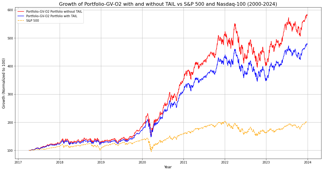
                               Alpha    Beta    Annualized Return  Volatility  Sharpe Ratio  Sortino Ratio  Max Drawdown  VaR 1M (95%)  VaR 6M (95%)  VaR 1Y (95%)  ES 1M (95%)  ES 6M (95%)  ES 1Y (95%)  R-Square
Portfolio-GV-O2 without TAIL 0.000622 1.086780      0.299328        0.243712     1.115379      1.433413      -0.350050     -0.106745     -0.347816     -0.577361    -0.142540    -0.435495    -0.701359         NaN
Portfolio-GV-O2 with TAIL    0.000560 0.912985      0.262029        0.208124     1.127078      1.462300      -0.300293     -0.093390     -0.304079     -0.504595    -0.124734    -0.380856    -0.613174         NaN
S&P 500                           NaN 1.000000      0.110526        0.196321     0.530843      0.634252      -0.339250     -0.124550     -0.341836     -0.519811    -0.174143    -0.463314    -0.691607    1.000000
Nasdaq-100                        NaN 1.000000      0.183523        0.241768     0.735701      0.939876      -0.355631     -0.157124     -0.443419     -0.685044    -0.218199    -0.593020    -0.896611    1.000000
Performance during recessions
recession_data = pd.read_csv('recession_indicator.csv', parse_dates=['DATE'])
recession_data["DATE"]
0 1854-12-01
1 1855-01-01
2 1855-02-01
3 1855-03-01
4 1855-04-01
...
2033 2024-05-01
2034 2024-06-01
2035 2024-07-01
2036 2024-08-01
2037 2024-09-01
Name: DATE, Length: 2038, dtype: datetime64[ns]import yfinance as yf
import numpy as np
import pandas as pd
import matplotlib.pyplot as plt
# Define the stocks and benchmark indices
stocks = ['ASML', 'TSLA', 'BRK-B', 'MSFT', 'ABBV', 'LMT']
benchmark_indices = ['^GSPC', '^NDX'] # S&P 500 and Nasdaq-100
# Download historical data
data = yf.download(stocks + benchmark_indices, start='2000-01-01', end='2024-01-01')['Close']
# Calculate daily returns
returns = data.pct_change()
returns.index = returns.index.tz_localize(None)
# Equal weights for portfolio
weights = np.array([0.15, 0.20, 0.25, 0.18, 0.10, 0.12])
# Calculate portfolio returns
portfolio_returns = (returns[stocks] * weights).sum(axis=1)
# Remove time zone information to ensure compatibility
portfolio_returns.index = portfolio_returns.index.tz_localize(None)
# Load recession periods from uploaded CSV file
recession_data = pd.read_csv('recession_indicator.csv', parse_dates=['DATE'])
recession_data.set_index('DATE', inplace=True)
recession_data.index = recession_data.index.tz_localize(None)
recession_daily = recession_data.reindex(pd.date_range(start=returns.index.min(),
end=returns.index.max(),
freq='D')).ffill()
# # Align the indices of returns and recession data
# recession_daily = recession_daily.reindex(returns.index, method='ffill')
# Filter returns for recession periods (only select days when recession is indicated)
recession_days_index = recession_daily[recession_daily['VALUE'] == 1].index
# Filter returns for recession periods (only select days when recession is indicated)
portfolio_recession_returns = portfolio_returns.loc[portfolio_returns.index.intersection(recession_days_index)]
# Define metrics functions
def annualized_return(returns):
compounded_growth = (1 + returns).prod()
n_years = len(returns) / 252
return compounded_growth ** (1 / n_years) - 1
def annualized_volatility(returns):
return returns.std() * np.sqrt(252)
def sharpe_ratio(returns, risk_free_rate=0.02):
excess_returns = returns - risk_free_rate / 252
return excess_returns.mean() / returns.std() * np.sqrt(252)
def sortino_ratio(returns, risk_free_rate=0.02):
downside_returns = returns[returns < 0]
downside_deviation = downside_returns.std() * np.sqrt(252)
return (returns.mean() - risk_free_rate / 252) / downside_deviation
def max_drawdown(returns):
cumulative = (1 + returns).cumprod()
peak = cumulative.cummax()
drawdown = (cumulative - peak) / peak
return drawdown.min()
# Calculate metrics for mini-fund portfolio during recession periods
portfolio_metrics_recession = {
'Annualized Return': annualized_return(portfolio_recession_returns),
'Volatility': annualized_volatility(portfolio_recession_returns),
'Sharpe Ratio': sharpe_ratio(portfolio_recession_returns),
'Sortino Ratio': sortino_ratio(portfolio_recession_returns),
'Max Drawdown': max_drawdown(portfolio_recession_returns)
}
# Calculate metrics for S&P 500 during recession periods
sp500_recession_returns = returns['^GSPC'].loc[returns.index.intersection(recession_days_index)]
sp500_metrics_recession = {
'Annualized Return': annualized_return(sp500_recession_returns),
'Volatility': annualized_volatility(sp500_recession_returns),
'Sharpe Ratio': sharpe_ratio(sp500_recession_returns),
'Sortino Ratio': sortino_ratio(sp500_recession_returns),
'Max Drawdown': max_drawdown(sp500_recession_returns)
}
# Calculate metrics for Nasdaq-100 during recession periods
ndx_recession_returns = returns['^NDX'].loc[returns.index.intersection(recession_days_index)]
ndx_metrics_recession = {
'Annualized Return': annualized_return(ndx_recession_returns),
'Volatility': annualized_volatility(ndx_recession_returns),
'Sharpe Ratio': sharpe_ratio(ndx_recession_returns),
'Sortino Ratio': sortino_ratio(ndx_recession_returns),
'Max Drawdown': max_drawdown(ndx_recession_returns)
}
# Combine results into a DataFrame
metrics_df_recession = pd.DataFrame([portfolio_metrics_recession, sp500_metrics_recession, ndx_metrics_recession], index=['Mini-Fund', 'S&P 500', 'Nasdaq-100'])
print("Portfolio Performance During Recession Periods:")
print(metrics_df_recession)
# Plot the cumulative returns during recession periods
cumulative_portfolio_returns_recession = (1 + portfolio_recession_returns).cumprod()
cumulative_sp500_returns_recession = (1 + sp500_recession_returns).cumprod()
cumulative_ndx_returns_recession = (1 + ndx_recession_returns).cumprod()
# Normalize cumulative returns to 100 for easy comparison
cumulative_portfolio_returns_normalized = cumulative_portfolio_returns_recession / cumulative_portfolio_returns_recession.iloc[0] * 100
cumulative_sp500_returns_normalized = cumulative_sp500_returns_recession / cumulative_sp500_returns_recession.iloc[0] * 100
cumulative_ndx_returns_normalized = cumulative_ndx_returns_recession / cumulative_ndx_returns_recession.iloc[0] * 100
# Plot the data
plt.figure(figsize=(15, 8))
# Plot the portfolio
plt.plot(cumulative_portfolio_returns_normalized, label='Mini-Fund Portfolio (Recession)', color='blue')
# Plot benchmark indices
plt.plot(cumulative_sp500_returns_normalized, label='S&P 500 (Recession)', linestyle='--', color='orange')
plt.plot(cumulative_ndx_returns_normalized, label='Nasdaq-100 (Recession)', linestyle='--', color='green')
# Add labels and title
plt.title('Growth of Portfolio-GV-O2 vs S&P 500 and Nasdaq-100 During Recession Periods', fontsize=16)
plt.xlabel('Year', fontsize=12)
plt.ylabel('Growth (Normalized to 100)', fontsize=12)
plt.legend(loc='upper left', fontsize=10)
# Show the plot
plt.grid(True)
plt.tight_layout()
plt.show()[*********************100%***********************] 8 of 8 completedPortfolio Performance During Recession Periods:
Annualized Return Volatility Sharpe Ratio Sortino Ratio Max Drawdown
Mini-Fund -0.031372 0.300771 -0.021338 -0.000109 -0.397179
S&P 500 -0.193706 0.385337 -0.417644 -0.002256 -0.600109
Nasdaq-100 -0.109028 0.460166 -0.065060 -0.000393 -0.613428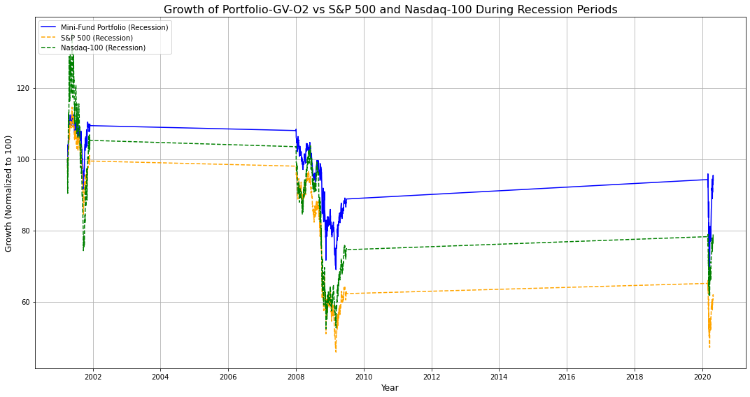
recession_dataimport yfinance as yf
import numpy as np
import pandas as pd
from scipy.optimize import minimize
# Download historical data for the stocks
stocks = ['ASML', 'NVDA', 'TSLA', 'BRK-B', 'MSFT']
data = yf.download(stocks, start='2010-01-01', end='2024-01-01')['Adj Close']
# Calculate daily returns
returns = data.pct_change().dropna()
# Define the function to calculate portfolio performance
def portfolio_performance(weights, mean_returns, cov_matrix, risk_free_rate=0.02):
returns = np.sum(mean_returns * weights) * 252
std = np.sqrt(np.dot(weights.T, np.dot(cov_matrix, weights))) * np.sqrt(252)
sharpe_ratio = (returns - risk_free_rate) / std
return returns, std, sharpe_ratio
# Define the objective function for optimization (negative Sharpe ratio)
def negative_sharpe_ratio(weights, mean_returns, cov_matrix, risk_free_rate=0.02):
returns, std, sharpe_ratio = portfolio_performance(weights, mean_returns, cov_matrix, risk_free_rate)
return -sharpe_ratio
# Constraints: sum of weights must be 1
def check_sum(weights):
return np.sum(weights) - 1
# Boundaries: weights between 0 and 1
bounds = tuple((0, 1) for stock in stocks)
# Initial guess (equal weight distribution)
initial_weights = np.array([1/len(stocks)] * len(stocks))
# Mean returns and covariance matrix
mean_returns = returns.mean()
cov_matrix = returns.cov()
# Optimization using minimize from scipy.optimize
optimal_solution = minimize(negative_sharpe_ratio, initial_weights, args=(mean_returns, cov_matrix),
method='SLSQP', bounds=bounds, constraints={'type': 'eq', 'fun': check_sum})
optimal_weights = optimal_solution.x
# Display optimal weights
optimal_weights_df = pd.DataFrame(optimal_weights, index=stocks, columns=['Optimal Weight'])
optimal_weights_percent = optimal_weights_df * 10000000000
# Display the weights in percentage form
print(optimal_weights_percent)
#print(optimal_weights_df)[*********************100%***********************] 5 of 5 completed Optimal Weight
ASML 1.639441e+01
NVDA 2.097931e-15
TSLA 2.852132e+01
BRK-B 3.240187e+01
MSFT 2.268240e+01import yfinance as yf
import numpy as np
import pandas as pd
from scipy.optimize import minimize
from scipy.stats import t
from arch import arch_model
from arch.__future__ import reindexing
stocks = ['ASML', 'TSLA', 'BRK-B', 'MSFT', 'ABBV', 'LMT']
protective_etf = ['TAIL']
# Combine stocks and protective ETF
all_assets = stocks + protective_etf
# Download historical data
data = yf.download(all_assets, start='2000-01-01', end='2024-01-01')['Adj Close']
# Calculate daily returns
returns = data.pct_change().dropna()
# Define the function to calculate portfolio performance
def portfolio_performance(weights, returns, risk_free_rate=0.02, confidence_level=0.95, forecast_volatility=True):
mean_returns = returns.mean()
cov_matrix = returns.cov()
portfolio_returns = np.dot(mean_returns, weights) * 252
portfolio_std = np.sqrt(np.dot(weights.T, np.dot(cov_matrix, weights))) * np.sqrt(252)
sharpe_ratio = (portfolio_returns - risk_free_rate) / portfolio_std
# Volatility calculation (GARCH(1,1) model)
if forecast_volatility:
am = arch_model(np.dot(returns, weights) * 100, vol='Garch', p=1, q=1, dist='t')
res = am.fit(disp='off')
std_dev_daily = res.forecast(horizon=1).variance.values[-1, 0] ** 0.5 / 100
else:
std_dev_daily = np.std(np.dot(returns, weights))
# Degrees of freedom for Student's t-distribution
df = 5 # Adjust as needed based on data
t_dist = t(df)
# t-score for the given confidence level (left tail)
t_score = t_dist.ppf(confidence_level)
# Time horizons in days
periods = {'1m': 21, '6m': 126}
var_list = []
es_list = []
for days in periods.values():
mean_return_period = portfolio_returns / 252 * days
std_dev_period = std_dev_daily * np.sqrt(days)
# VaR Calculation
var = - (mean_return_period + t_score * std_dev_period)
# ES Calculation
es_factor = (t_dist.pdf(t_score) / (1 - confidence_level)) * ((df + t_score**2) / (df - 1))
es = - (mean_return_period + es_factor * std_dev_period)
var_list.append(var)
es_list.append(es)
var_1m, var_6m = var_list
es_1m, es_6m = es_list
return portfolio_returns, portfolio_std, sharpe_ratio, var_1m, var_6m, es_1m, es_6m
# Define the objective function for optimization
def objective(weights, returns, risk_free_rate=0.02, confidence_level=0.95):
portfolio_returns, portfolio_std, sharpe_ratio, var_1m, var_6m, es_1m, es_6m = portfolio_performance(weights, returns, risk_free_rate, confidence_level)
# Weights for multi-objective optimization
w_sharpe, w_var, w_es = 1.0, 0.5, 0.5 # Adjust these weights as per preference
# Objective value to minimize: negative Sharpe ratio + VaR + ES
objective_value = (
w_sharpe * -sharpe_ratio + # Maximizing Sharpe Ratio by minimizing its negative
w_var * (var_1m + var_6m) + # Minimize VaR (1 month and 6 months)
w_es * (es_1m + es_6m) # Minimize ES (1 month and 6 months)
)
return objective_value
# Constraints: sum of weights must be 1
def check_sum(weights):
return np.sum(weights) - 1
# Boundaries: weights between 0 and 1
bounds = tuple((0, 1) for _ in all_assets)
# Initial guess (equal weight distribution)
# initial_weights = np.array([1 / len(all_assets)] * len(all_assets))
initial_weights = np.array([0.13, 0.18, 0.22, 0.16, 0.10, 0.11, 0.10]) # Added 10% weight to TAIL
# Optimization using minimize from scipy.optimize
optimal_solution = minimize(objective, initial_weights, args=(returns),
method='SLSQP', bounds=bounds, constraints={'type': 'eq', 'fun': check_sum})
optimal_weights = optimal_solution.x
# Display optimal weights
optimal_weights_df = pd.DataFrame(optimal_weights, index=all_assets, columns=['Optimal Weight'])
#optimal_weights_percent = optimal_weights_df * 100
# Display the weights in percentage form
print(optimal_weights_df)[*********************100%***********************] 7 of 7 completed Optimal Weight
ASML 0.107482
TSLA 0.182479
BRK-B 0.183304
MSFT 0.194264
ABBV 0.083253
LMT 0.091662
TAIL 0.157556
**************************************************************************************
**************************************************************************************stocks = ['ASML', 'TSLA', 'BRK-B', 'MSFT', 'ABBV', 'LMT']
benchmark_indices = ['^GSPC', '^NDX'] # S&P 500 and Nasdaq-100
protective_etf = ['TAIL']
# Download historical data
data = yf.download(stocks + benchmark_indices + protective_etf, start='2000-01-01', end='2024-01-01')['Adj Close']
# Calculate daily returns
returns = data.pct_change().dropna()
# Calculate portfolio returns with TAIL
portfolio_returns_with_tail = (returns[stocks + protective_etf] * optimal_weights).sum(axis=1)
# Calculate cumulative returns
cumulative_portfolio_returns_without_tail = (1 + portfolio_returns_without_tail).cumprod()
cumulative_portfolio_returns_with_tail = (1 + portfolio_returns_with_tail).cumprod()
cumulative_sp500_returns = (1 + returns['^GSPC']).cumprod()
cumulative_ndx_returns = (1 + returns['^NDX']).cumprod()
# Define metrics functions
def annualized_return(returns, periods_per_year=252):
compounded_growth = (1 + returns).prod()
n_periods = returns.count()
return compounded_growth ** (periods_per_year / n_periods) - 1
def annualized_volatility(returns, periods_per_year=252):
return returns.std() * np.sqrt(periods_per_year)
def sharpe_ratio(returns, risk_free_rate=0.02, periods_per_year=252):
excess_returns = returns - risk_free_rate / periods_per_year
return excess_returns.mean() / returns.std() * np.sqrt(periods_per_year)
def sortino_ratio(returns, risk_free_rate=0.02, periods_per_year=252):
downside_returns = returns[returns < 0]
excess_returns = returns - risk_free_rate / periods_per_year
return excess_returns.mean() / downside_returns.std() * np.sqrt(periods_per_year)
def max_drawdown(returns):
cumulative_returns = (1 + returns).cumprod()
peak = cumulative_returns.expanding(min_periods=1).max()
drawdown = (cumulative_returns - peak) / peak
return drawdown.min()
def alpha_beta(returns, benchmark_returns):
cov_matrix = np.cov(returns, benchmark_returns)
beta = cov_matrix[0, 1] / cov_matrix[1, 1]
alpha = returns.mean() - beta * benchmark_returns.mean()
return alpha, beta
def var_es(returns, confidence_level=0.95, forecast_volatility=False):
# Calculate the mean return (daily)
mean_return_daily = returns.mean()
# Volatility calculation
if forecast_volatility:
# Fit GARCH(1,1) model to the return series
am = arch_model(returns * 100, vol='Garch', p=1, q=1, dist='t')
res = am.fit(disp='off')
# Use last forecasted volatility (scaled back to decimal)
std_dev_daily = res.forecast(horizon=1).variance.values[-1, 0] ** 0.5 / 100
else:
# Use historical standard deviation
std_dev_daily = returns.std()
# Degrees of freedom for Student's t-distribution
df = 5 # Adjust as needed based on data
t_dist = t(df)
# t-score for the given confidence level (left tail)
t_score = t_dist.ppf(confidence_level)
# Time horizons in days
periods = {'1m': 21, '6m': 126, '1y': 252}
var_list = []
es_list = []
for days in periods.values():
mean_return_period = mean_return_daily * days
std_dev_period = std_dev_daily * np.sqrt(days)
# VaR Calculation
var = - (mean_return_period + t_score * std_dev_period)
# ES Calculation
es_factor = (t_dist.pdf(t_score) / (1 - confidence_level)) * ((df + t_score**2) / (df - 1))
es = - (mean_return_period + es_factor * std_dev_period)
var_list.append(var)
es_list.append(es)
var_1m, var_6m, var_1y = var_list
es_1m, es_6m, es_1y = es_list
return var_1m, var_6m, var_1y, es_1m, es_6m, es_1y
# Calculate Alpha, Beta, VaR, and ES for portfolios and benchmarks
market_returns = returns['^GSPC']
alpha_portfolio_without_tail, beta_portfolio_without_tail = alpha_beta(portfolio_returns_without_tail, market_returns)
alpha_portfolio_with_tail, beta_portfolio_with_tail = alpha_beta(portfolio_returns_with_tail, market_returns)
var_1m_without_tail, var_6m_without_tail, var_1y_without_tail, es_1m_without_tail, es_6m_without_tail, es_1y_without_tail = var_es(portfolio_returns_without_tail, forecast_volatility=True)
var_1m_with_tail, var_6m_with_tail, var_1y_with_tail, es_1m_with_tail, es_6m_with_tail, es_1y_with_tail = var_es(portfolio_returns_with_tail, forecast_volatility=True)
# Calculate metrics for mini-fund portfolio without TAIL
portfolio_metrics_without_tail = {
'Alpha': alpha_portfolio_without_tail,
'Beta': beta_portfolio_without_tail,
'Annualized Return': annualized_return(portfolio_returns_without_tail),
'Volatility': annualized_volatility(portfolio_returns_without_tail),
'Sharpe Ratio': sharpe_ratio(portfolio_returns_without_tail),
'Sortino Ratio': sortino_ratio(portfolio_returns_without_tail),
'Max Drawdown': max_drawdown(portfolio_returns_without_tail),
'VaR 1M (95%)': var_1m_without_tail,
'VaR 6M (95%)': var_6m_without_tail,
'VaR 1Y (95%)': var_1y_without_tail,
'ES 1M (95%)': es_1m_without_tail,
'ES 6M (95%)': es_6m_without_tail,
'ES 1Y (95%)': es_1y_without_tail
}
# Calculate metrics for mini-fund portfolio with TAIL
portfolio_metrics_with_tail = {
'Alpha': alpha_portfolio_with_tail,
'Beta': beta_portfolio_with_tail,
'Annualized Return': annualized_return(portfolio_returns_with_tail),
'Volatility': annualized_volatility(portfolio_returns_with_tail),
'Sharpe Ratio': sharpe_ratio(portfolio_returns_with_tail),
'Sortino Ratio': sortino_ratio(portfolio_returns_with_tail),
'Max Drawdown': max_drawdown(portfolio_returns_with_tail),
'VaR 1M (95%)': var_1m_with_tail,
'VaR 6M (95%)': var_6m_with_tail,
'VaR 1Y (95%)': var_1y_with_tail,
'ES 1M (95%)': es_1m_with_tail,
'ES 6M (95%)': es_6m_with_tail,
'ES 1Y (95%)': es_1y_with_tail
}
# Calculate metrics for S&P 500
sp500_metrics = {
'Beta': 1,
'R-Square': 1,
'Annualized Return': annualized_return(returns['^GSPC']),
'Volatility': annualized_volatility(returns['^GSPC']),
'Sharpe Ratio': sharpe_ratio(returns['^GSPC']),
'Sortino Ratio': sortino_ratio(returns['^GSPC']),
'Max Drawdown': max_drawdown(returns['^GSPC']),
'VaR 1M (95%)': var_es(returns['^GSPC'])[0],
'VaR 6M (95%)': var_es(returns['^GSPC'])[1],
'VaR 1Y (95%)': var_es(returns['^GSPC'])[2],
'ES 1M (95%)': var_es(returns['^GSPC'])[3],
'ES 6M (95%)': var_es(returns['^GSPC'])[4],
'ES 1Y (95%)': var_es(returns['^GSPC'])[5]
}
# Normalize cumulative returns to 100 for easy comparison
cumulative_portfolio_returns_without_tail_normalized = cumulative_portfolio_returns_without_tail / cumulative_portfolio_returns_without_tail.iloc[0] * 100
cumulative_portfolio_returns_with_tail_normalized = cumulative_portfolio_returns_with_tail / cumulative_portfolio_returns_with_tail.iloc[0] * 100
cumulative_sp500_returns_normalized = cumulative_sp500_returns / cumulative_sp500_returns.iloc[0] * 100
# Plot the data
plt.figure(figsize=(15, 8))
# Plot the portfolio without TAIL
plt.plot(cumulative_portfolio_returns_without_tail_normalized, label='Portfolio-GV-O2', color='red')
# Plot the portfolio with TAIL
plt.plot(cumulative_portfolio_returns_with_tail_normalized, label='Portfolio-GV-TAIL-O', color='blue')
# Plot benchmark indices
plt.plot(cumulative_sp500_returns_normalized, label='S&P 500', linestyle='--', color='orange')
# Add labels and title
plt.title('Growth of Portfolio-GV-TAIL-O vs Portfolio-GV-O2 (no TAIL) vs S&P 500 and Nasdaq-100 (2000-2024)', fontsize=16)
plt.xlabel('Year', fontsize=12)
plt.ylabel('Growth (Normalized to 100)', fontsize=12)
plt.legend(loc='upper left', fontsize=10)
# Show the plot
plt.grid(True)
plt.tight_layout()
plt.show()
# Combine results into a DataFrame
metrics_df = pd.DataFrame([portfolio_metrics_without_tail, portfolio_metrics_with_tail, sp500_metrics, ndx_metrics],
index=['Portfolio-GV-O2', 'Portfolio-GV-TAIL-O', 'S&P 500', 'Nasdaq-100'])
# Adjust display settings to show all columns without wrapping
pd.set_option('display.max_columns', None) # Show all columns
pd.set_option('display.expand_frame_repr', False) # Prevent DataFrame from wrapping
pd.set_option('display.width', 1000) # Set width to large enough value
pd.set_option('display.colheader_justify', 'center') # Center align the headers
pd.set_option('display.float_format', '{:.6f}'.format) # Format float to 6 decimal places
print(metrics_df)[*********************100%***********************] 9 of 9 completed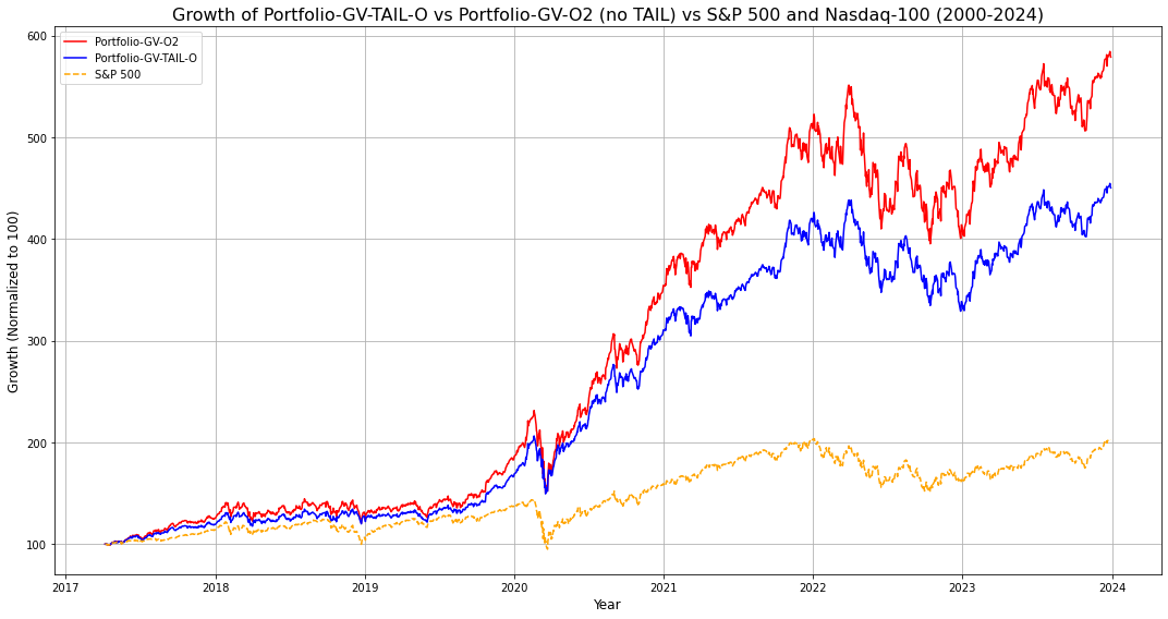
                      Alpha    Beta    Annualized Return  Volatility  Sharpe Ratio  Sortino Ratio  Max Drawdown  VaR 1M (95%)  VaR 6M (95%)  VaR 1Y (95%)  ES 1M (95%)  ES 6M (95%)  ES 1Y (95%)  R-Square
Portfolio-GV-O2     0.000622 1.086780      0.299328        0.243712     1.115379      1.433413      -0.350050     -0.106745     -0.347816     -0.577361    -0.142540    -0.435495    -0.701359         NaN
Portfolio-GV-TAIL-O 0.000554 0.837946      0.251487        0.196279     1.139983      1.500943      -0.275660     -0.088748     -0.289508     -0.480820    -0.118467    -0.362305    -0.583771         NaN
S&P 500                  NaN 1.000000      0.110526        0.196321     0.530843      0.634252      -0.339250     -0.124550     -0.341836     -0.519811    -0.174143    -0.463314    -0.691607    1.000000
Nasdaq-100               NaN 1.000000      0.183523        0.241768     0.735701      0.939876      -0.355631     -0.157124     -0.443419     -0.685044    -0.218199    -0.593020    -0.896611    1.000000
CWARP
https://docsend.com/view/teaqrcewe7ht423x
import numpy as np
import pandas as pd
import yfinance as yf
import matplotlib.pyplot as plt

# Define a function to calculate Sortino Ratio
# Rp: Return of Portfolio, Rf: Risk-Free Rate, sigma_dp: Downside Deviation of Portfolio
def sortino_ratio(Rp, Rf, sigma_dp):
    return (Rp - Rf) / sigma_dp

# Define a function to calculate Return to Max Drawdown (RMDD)
# Rp: Return of Portfolio, Lp: Trough value of Replacement Portfolio, Pp: Peak value of Replacement Portfolio
def return_to_max_drawdown(Rp, Lp, Pp):
    return (Rp - Rf) / ((Lp - Pp) / Pp)

# Define the CWARP Calculation Function
# Sn: Sortino Ratio of New Portfolio, Sp: Sortino Ratio of Replacement Portfolio
# RMDDn: Return to Max Drawdown of New Portfolio, RMDDp: Return to Max Drawdown of Replacement Portfolio
def cwarp_calculation(Sn, Sp, RMDDn, RMDDp):
    return (np.sqrt((Sn / Sp) * (RMDDn / RMDDp)) - 1) * 100

# Download historical data for portfolio and benchmarks
stocks = ['ASML', 'TSLA', 'BRK-B', 'MSFT', 'ABBV', 'LMT']
benchmark_indices = ['^GSPC', '^NDX']  # S&P 500 and Nasdaq-100
data = yf.download(stocks + benchmark_indices, start='2000-01-01', end='2024-01-01')['Adj Close']

# Calculate daily returns
returns = data.pct_change().dropna()

# Equal weights for portfolio
weights = np.array([0.15, 0.20, 0.25, 0.18, 0.10, 0.12])

# Calculate portfolio returns
portfolio_returns = (returns[stocks] * weights).sum(axis=1)

# Risk-free rate (assumed)
Rf = 0.02 / 252  # Annual risk-free rate divided by trading days

# Calculate Sortino Ratios for Portfolio, S&P 500, and Nasdaq-100
portfolio_downside_std = portfolio_returns[portfolio_returns < 0].std()
sp500_downside_std = returns['^GSPC'][returns['^GSPC'] < 0].std()
ndx_downside_std = returns['^NDX'][returns['^NDX'] < 0].std()

Sp_portfolio = sortino_ratio(portfolio_returns.mean(), Rf, portfolio_downside_std)
Sp_sp500 = sortino_ratio(returns['^GSPC'].mean(), Rf, sp500_downside_std)
Sp_ndx = sortino_ratio(returns['^NDX'].mean(), Rf, ndx_downside_std)

# Calculate Return to Max Drawdowns for Portfolio, S&P 500, and Nasdaq-100
portfolio_peak = portfolio_returns.cummax()
portfolio_drawdown = (portfolio_returns - portfolio_peak) / portfolio_peak
Lp_portfolio = portfolio_drawdown.min()
Pp_portfolio = portfolio_peak.max()
RMDD_portfolio = return_to_max_drawdown(portfolio_returns.mean(), Lp_portfolio, Pp_portfolio)

sp500_peak = returns['^GSPC'].cummax()
sp500_drawdown = (returns['^GSPC'] - sp500_peak) / sp500_peak
Lp_sp500 = sp500_drawdown.min()
Pp_sp500 = sp500_peak.max()
RMDD_sp500 = return_to_max_drawdown(returns['^GSPC'].mean(), Lp_sp500, Pp_sp500)

ndx_peak = returns['^NDX'].cummax()
ndx_drawdown = (returns['^NDX'] - ndx_peak) / ndx_peak
Lp_ndx = ndx_drawdown.min()
Pp_ndx = ndx_peak.max()
RMDD_ndx = return_to_max_drawdown(returns['^NDX'].mean(), Lp_ndx, Pp_ndx)

# Calculate CWARP for Portfolio vs S&P 500 and Nasdaq-100
cwarp_portfolio_sp500 = cwarp_calculation(Sp_portfolio, Sp_sp500, RMDD_portfolio, RMDD_sp500)
cwarp_portfolio_ndx = cwarp_calculation(Sp_portfolio, Sp_ndx, RMDD_portfolio, RMDD_ndx)

print(f"CWARP Value (Portfolio vs S&P 500): {cwarp_portfolio_sp500}")
print(f"CWARP Value (Portfolio vs Nasdaq-100): {cwarp_portfolio_ndx}")
[*********************100%***********************] 8 of 8 completedCWARP Value (Portfolio vs S&P 500): 162.3071593499393
CWARP Value (Portfolio vs Nasdaq-100): 78.84851594077611