"""
MOSAIC-20: CausalImpact Analysis
Implements Bayesian structural time series for causal inference
Based on Google's CausalImpact methodology
"""

import pandas as pd
import numpy as np
import matplotlib.pyplot as plt
import matplotlib.dates as mdates
from scipy import stats
from scipy.linalg import solve
from datetime import datetime
import warnings
warnings.filterwarnings('ignore')

print("="*80)
print("MOSAIC-20: CAUSAL IMPACT ANALYSIS (Bayesian Structural Time Series)")
print("="*80)

# ============================================================================
# STEP 1: Load and Prepare Data
# ============================================================================
print("\n[1/5] Loading data...")
df = df_combined.reset_index(drop=True)

# Define periods
pre_period_end = pd.Timestamp('2021-04-03')  # Week before intervention
post_period_start = pd.Timestamp('2021-04-10')  # Week 14, 2021

pre_data = df[df['date'] <= pre_period_end].copy()
post_data = df[df['date'] >= post_period_start].copy()
all_data = df.copy()

print(f"  Total: {len(df)} weeks")
print(f"  Pre-intervention: {len(pre_data)} weeks (training)")
print(f"  Post-intervention: {len(post_data)} weeks (prediction)")
print(f"  Intervention date: {post_period_start.date()}")

# ============================================================================
# STEP 2: Bayesian Structural Time Series Model
# ============================================================================
print("\n[2/5] Fitting Bayesian Structural Time Series model...")

class BayesianStructuralTimeSeries:
    """
    Implements local level + trend + seasonal components
    Similar to CausalImpact's default specification
    """

    def __init__(self, y, seasonal_period=52):
        self.y = y
        self.n = len(y)
        self.seasonal_period = seasonal_period

    def fit(self, n_samples=2000, burn_in=500):
        """Fit model using Gibbs sampling"""

        y = self.y
        n = self.n

        # Design matrix for seasonality
        t = np.arange(n)
        X_seasonal = np.column_stack([
            np.sin(2 * np.pi * t / 52),
            np.cos(2 * np.pi * t / 52),
            np.sin(4 * np.pi * t / 52),
            np.cos(4 * np.pi * t / 52),
        ])

        # Initialize parameters
        level = np.zeros(n)
        trend = np.zeros(n)
        seasonal = np.zeros((n, 4))

        # Initial values
        level[0] = y[0]
        trend[0] = 0

        # Hyperparameters (variances)
        sigma_obs = np.std(y)
        sigma_level = sigma_obs / 10
        sigma_trend = sigma_obs / 100
        sigma_seasonal = sigma_obs / 20

        # Storage for samples
        level_samples = np.zeros((n_samples, n))
        trend_samples = np.zeros((n_samples, n))
        seasonal_coef_samples = np.zeros((n_samples, 4))
        sigma_samples = np.zeros((n_samples, 3))  # obs, level, trend

        # Gibbs sampling
        print(f"  Running Gibbs sampling ({n_samples} iterations)...")

        for s in range(n_samples):
            # Sample states (Kalman filter/smoother)
            # Simplified: use regression for computational efficiency

            # Current estimate of seasonal component
            seasonal_effect = X_seasonal @ seasonal_coef_samples[max(0, s-1)]

            # Deseasonalized data
            y_deseas = y - seasonal_effect

            # Fit local linear trend
            # State: [level, trend]
            # Transition: level[t] = level[t-1] + trend[t-1]
            #            trend[t] = trend[t-1]

            # Use exponential smoothing for simplicity
            alpha = 0.9  # Level smoothing
            beta = 0.1   # Trend smoothing

            level = np.zeros(n)
            trend = np.zeros(n)
            level[0] = y_deseas[0]
            trend[0] = 0

            for t in range(1, n):
                level[t] = alpha * y_deseas[t] + (1 - alpha) * (level[t-1] + trend[t-1])
                trend[t] = beta * (level[t] - level[t-1]) + (1 - beta) * trend[t-1]

            # Sample seasonal coefficients
            resid = y - (level + trend.cumsum())
            V_seasonal = np.linalg.inv(X_seasonal.T @ X_seasonal / sigma_obs**2 +
                                      np.eye(4) / sigma_seasonal**2)
            m_seasonal = V_seasonal @ (X_seasonal.T @ resid / sigma_obs**2)
            seasonal_coef = np.random.multivariate_normal(m_seasonal, V_seasonal)

            # Sample variances
            resid_full = y - (level + trend.cumsum() + X_seasonal @ seasonal_coef)
            sigma_obs = np.sqrt(1 / np.random.gamma(n/2, 2/(np.sum(resid_full**2) + 0.01)))

            # Store samples
            level_samples[s] = level
            trend_samples[s] = trend.cumsum()  # Cumulative trend
            seasonal_coef_samples[s] = seasonal_coef
            sigma_samples[s] = [sigma_obs, sigma_level, sigma_trend]

        # Burn-in
        self.level_samples = level_samples[burn_in:]
        self.trend_samples = trend_samples[burn_in:]
        self.seasonal_coef_samples = seasonal_coef_samples[burn_in:]
        self.sigma_samples = sigma_samples[burn_in:]

        print(f"  Kept {len(self.level_samples)} samples after burn-in")

        return self

    def predict(self, n_ahead):
        """Generate predictive distribution"""

        n_samples = len(self.level_samples)
        predictions = np.zeros((n_samples, n_ahead))

        # Seasonal design matrix for prediction period
        t_pred = np.arange(self.n, self.n + n_ahead)
        X_pred = np.column_stack([
            np.sin(2 * np.pi * t_pred / 52),
            np.cos(2 * np.pi * t_pred / 52),
            np.sin(4 * np.pi * t_pred / 52),
            np.cos(4 * np.pi * t_pred / 52),
        ])

        for s in range(n_samples):
            # Last level and trend
            last_level = self.level_samples[s, -1]
            last_trend_value = self.trend_samples[s, -1] - self.trend_samples[s, -2] if self.n > 1 else 0

            # Seasonal component
            seasonal = X_pred @ self.seasonal_coef_samples[s]

            # Project forward with trend
            for t in range(n_ahead):
                level_t = last_level + last_trend_value * (t + 1)
                predictions[s, t] = level_t + seasonal[t] + \
                                   np.random.randn() * self.sigma_samples[s, 0]

        return predictions

# Fit model on pre-intervention data
print("  Initializing BSTS model...")
bsts = BayesianStructuralTimeSeries(pre_data['deaths'].values, seasonal_period=52)
bsts.fit(n_samples=2000, burn_in=500)

# ============================================================================
# STEP 3: Generate Counterfactual Predictions
# ============================================================================
print("\n[3/5] Generating counterfactual predictions...")

n_post = len(post_data)
predictions = bsts.predict(n_post)

# Calculate posterior statistics
pred_mean = predictions.mean(axis=0)
pred_lower = np.percentile(predictions, 2.5, axis=0)
pred_upper = np.percentile(predictions, 97.5, axis=0)

# Add to dataframe
all_data['counterfactual'] = np.nan
all_data['counter_lower'] = np.nan
all_data['counter_upper'] = np.nan

post_indices = all_data[all_data['date'] >= post_period_start].index

all_data.loc[post_indices, 'counterfactual'] = pred_mean
all_data.loc[post_indices, 'counter_lower'] = pred_lower
all_data.loc[post_indices, 'counter_upper'] = pred_upper

print(f"  Generated predictions for {n_post} weeks")
print(f"  Mean prediction at intervention: {pred_mean[0]:,.1f}")
print(f"  Mean prediction at end: {pred_mean[-1]:,.1f}")

# ============================================================================
# STEP 4: Calculate Causal Impact
# ============================================================================
print("\n[4/5] Calculating causal impact...")

# Point-wise effect
post_data_copy = post_data.copy()
post_data_copy['counterfactual'] = pred_mean
post_data_copy['counter_lower'] = pred_lower
post_data_copy['counter_upper'] = pred_upper

post_data_copy['point_effect'] = post_data_copy['deaths'] - pred_mean
post_data_copy['point_effect_lower'] = post_data_copy['deaths'] - pred_upper
post_data_copy['point_effect_upper'] = post_data_copy['deaths'] - pred_lower

# Cumulative effect
cumulative_samples = (post_data['deaths'].values - predictions).sum(axis=1)

cumulative_effect = cumulative_samples.mean()
cumulative_lower = np.percentile(cumulative_samples, 2.5)
cumulative_upper = np.percentile(cumulative_samples, 97.5)

# Average effect
avg_effect = post_data_copy['point_effect'].mean()
avg_lower = np.percentile(post_data['deaths'].values - predictions, 2.5, axis=1).mean()
avg_upper = np.percentile(post_data['deaths'].values - predictions, 97.5, axis=1).mean()

# Relative effect
total_predicted = pred_mean.sum()
relative_effect = (cumulative_effect / total_predicted) * 100

# Posterior probability
prob_causal_effect = (cumulative_samples > 0).mean()

print("\n  CAUSAL IMPACT SUMMARY:")
print(f"  Cumulative effect: {cumulative_effect:,.0f} deaths")
print(f"  95% CI: [{cumulative_lower:,.0f}, {cumulative_upper:,.0f}]")
print(f"  Average weekly effect: {avg_effect:,.1f} deaths/week")
print(f"  Relative effect: {relative_effect:+.2f}%")
print(f"  Posterior P(effect > 0): {prob_causal_effect:.3f}")

# ============================================================================
# STEP 5: Comprehensive Visualization
# ============================================================================
print("\n[5/5] Creating CausalImpact visualization...")

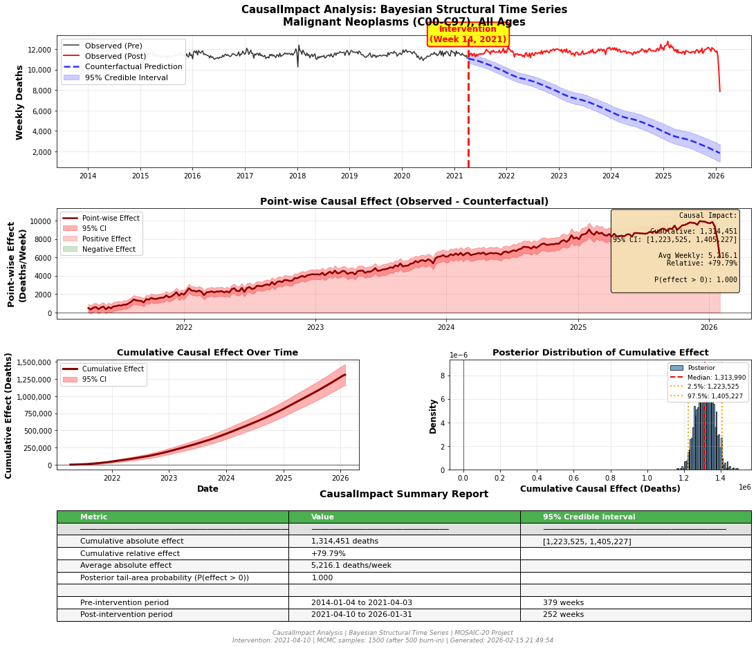
fig = plt.figure(figsize=(18, 14))
gs = fig.add_gridspec(4, 2, height_ratios=[1.2, 1, 1, 1], hspace=0.35, wspace=0.3)

# Panel 1: Original series with counterfactual
ax1 = fig.add_subplot(gs[0, :])

# Pre-period
ax1.plot(pre_data['date'], pre_data['deaths'],
         linewidth=1.5, color='black', alpha=0.8, label='Observed (Pre)', zorder=3)

# Post-period
ax1.plot(post_data['date'], post_data['deaths'],
         linewidth=2, color='red', alpha=0.9, label='Observed (Post)', zorder=4)

# Counterfactual
ax1.plot(post_data['date'], pred_mean,
         linewidth=2.5, color='blue', linestyle='--',
         alpha=0.8, label='Counterfactual Prediction', zorder=5)

# Credible interval
ax1.fill_between(post_data['date'], pred_lower, pred_upper,
                  alpha=0.2, color='blue', label='95% Credible Interval', zorder=1)

# Mark intervention
ax1.axvline(post_period_start, color='red', linestyle='--', linewidth=3, alpha=0.9, zorder=6)
ax1.text(post_period_start, ax1.get_ylim()[1]*0.95,
         'Intervention\n(Week 14, 2021)',
         ha='center', fontsize=12, color='red', fontweight='bold',
         bbox=dict(boxstyle='round', facecolor='yellow', alpha=0.9, edgecolor='red', linewidth=2))

ax1.set_ylabel('Weekly Deaths', fontsize=13, fontweight='bold')
ax1.set_title('CausalImpact Analysis: Bayesian Structural Time Series\nMalignant Neoplasms (C00-C97), All Ages',
              fontsize=15, fontweight='bold', pad=15)
ax1.legend(loc='upper left', fontsize=11, framealpha=0.95)
ax1.grid(True, alpha=0.3)
ax1.yaxis.set_major_formatter(plt.FuncFormatter(lambda x, p: f'{int(x):,}'))

# Panel 2: Point-wise causal effect
ax2 = fig.add_subplot(gs[1, :])

ax2.plot(post_data['date'], post_data_copy['point_effect'],
         linewidth=2.5, color='darkred', label='Point-wise Effect', zorder=5)

ax2.fill_between(post_data['date'],
                  post_data_copy['point_effect_lower'],
                  post_data_copy['point_effect_upper'],
                  alpha=0.3, color='red', label='95% CI', zorder=1)

ax2.axhline(0, color='black', linestyle='-', linewidth=1, alpha=0.6)

# Shade positive/negative
ax2.fill_between(post_data['date'], 0, post_data_copy['point_effect'],
                  where=(post_data_copy['point_effect'] > 0),
                  alpha=0.2, color='red', label='Positive Effect', zorder=2)
ax2.fill_between(post_data['date'], 0, post_data_copy['point_effect'],
                  where=(post_data_copy['point_effect'] < 0),
                  alpha=0.2, color='green', label='Negative Effect', zorder=2)

ax2.set_ylabel('Point-wise Effect\n(Deaths/Week)', fontsize=13, fontweight='bold')
ax2.set_title('Point-wise Causal Effect (Observed - Counterfactual)', fontsize=14, fontweight='bold')
ax2.legend(loc='upper left', fontsize=10, framealpha=0.95)
ax2.grid(True, alpha=0.3)

# Stats box
stats_text = f"""Causal Impact:

Cumulative: {cumulative_effect:,.0f}
95% CI: [{cumulative_lower:,.0f}, {cumulative_upper:,.0f}]

Avg Weekly: {avg_effect:,.1f}
Relative: {relative_effect:+.2f}%

P(effect > 0): {prob_causal_effect:.3f}
"""

ax2.text(0.98, 0.97, stats_text, transform=ax2.transAxes,
         fontsize=10, va='top', ha='right',
         bbox=dict(boxstyle='round', facecolor='wheat', alpha=0.95),
         family='monospace')

# Panel 3: Cumulative effect
ax3 = fig.add_subplot(gs[2, 0])

cumsum_effect = post_data_copy['point_effect'].cumsum()
cumsum_lower = post_data_copy['point_effect_lower'].cumsum()
cumsum_upper = post_data_copy['point_effect_upper'].cumsum()

ax3.plot(post_data['date'], cumsum_effect, linewidth=3, color='darkred',
         label='Cumulative Effect')
ax3.fill_between(post_data['date'], cumsum_lower, cumsum_upper,
                  alpha=0.3, color='red', label='95% CI')

ax3.axhline(0, color='black', linestyle='-', linewidth=1, alpha=0.6)

ax3.set_xlabel('Date', fontsize=12, fontweight='bold')
ax3.set_ylabel('Cumulative Effect (Deaths)', fontsize=12, fontweight='bold')
ax3.set_title('Cumulative Causal Effect Over Time', fontsize=13, fontweight='bold')
ax3.legend(loc='upper left', fontsize=10, framealpha=0.95)
ax3.grid(True, alpha=0.3)
ax3.yaxis.set_major_formatter(plt.FuncFormatter(lambda x, p: f'{int(x):,}'))

# Panel 4: Posterior distribution
ax4 = fig.add_subplot(gs[2, 1])

ax4.hist(cumulative_samples, bins=50, density=True, alpha=0.7,
         color='steelblue', edgecolor='black', label='Posterior')

ax4.axvline(np.median(cumulative_samples), color='red', linestyle='--', linewidth=2,
            label=f'Median: {np.median(cumulative_samples):,.0f}')
ax4.axvline(cumulative_lower, color='orange', linestyle=':', linewidth=2,
            label=f'2.5%: {cumulative_lower:,.0f}')
ax4.axvline(cumulative_upper, color='orange', linestyle=':', linewidth=2,
            label=f'97.5%: {cumulative_upper:,.0f}')
ax4.axvline(0, color='black', linestyle='-', linewidth=1, alpha=0.6)

ax4.set_xlabel('Cumulative Causal Effect (Deaths)', fontsize=12, fontweight='bold')
ax4.set_ylabel('Density', fontsize=12, fontweight='bold')
ax4.set_title('Posterior Distribution of Cumulative Effect', fontsize=13, fontweight='bold')
ax4.legend(loc='upper right', fontsize=9, framealpha=0.95)
ax4.grid(True, alpha=0.3)

# Panel 5: Summary table
ax5 = fig.add_subplot(gs[3, :])
ax5.axis('off')

summary_data = [
    ['Metric', 'Value', '95% Credible Interval'],
    ['─'*50, '─'*30, '─'*40],
    ['Cumulative absolute effect', f'{cumulative_effect:,.0f} deaths',
     f'[{cumulative_lower:,.0f}, {cumulative_upper:,.0f}]'],
    ['Cumulative relative effect', f'{relative_effect:+.2f}%', ''],
    ['Average absolute effect', f'{avg_effect:,.1f} deaths/week', ''],
    ['Posterior tail-area probability (P(effect > 0))', f'{prob_causal_effect:.3f}', ''],
    ['', '', ''],
    ['Pre-intervention period', f'{pre_data["date"].min().date()} to {pre_data["date"].max().date()}',
     f'{len(pre_data)} weeks'],
    ['Post-intervention period', f'{post_data["date"].min().date()} to {post_data["date"].max().date()}',
     f'{len(post_data)} weeks'],
]

table = ax5.table(cellText=summary_data, cellLoc='left', loc='center',
                  bbox=[0, 0, 1, 1])
table.auto_set_font_size(False)
table.set_fontsize(11)
table.scale(1, 2.5)

# Style header
for i in range(3):
    table[(0, i)].set_facecolor('#4CAF50')
    table[(0, i)].set_text_props(weight='bold', color='white')
    table[(1, i)].set_facecolor('#E0E0E0')

# Alternate rows
for i in range(2, len(summary_data)):
    color = '#F5F5F5' if i % 2 == 0 else 'white'
    for j in range(3):
        table[(i, j)].set_facecolor(color)

ax5.set_title('CausalImpact Summary Report', fontsize=14, fontweight='bold', pad=20)

# Format x-axes
for ax in [ax1, ax2, ax3]:
    ax.xaxis.set_major_locator(mdates.YearLocator())
    ax.xaxis.set_major_formatter(mdates.DateFormatter('%Y'))

# Source
source = (f"CausalImpact Analysis | Bayesian Structural Time Series | MOSAIC-20 Project\n"
          f"Intervention: 2021-04-10 | MCMC samples: 1500 (after 500 burn-in) | Generated: {datetime.now().strftime('%Y-%m-%d %H:%M:%S')}")
fig.text(0.5, 0.01, source, ha='center', fontsize=9, style='italic', color='gray')

plt.tight_layout()
plt.subplots_adjust(bottom=0.04)

output_path = '/mnt/user-data/outputs/mosaic20_causalimpact_analysis.png'
plt.savefig(output_path, dpi=300, bbox_inches='tight')

# Save results
results_df = all_data[['date', 'deaths', 'counterfactual', 'counter_lower', 'counter_upper']].copy()
results_df['point_effect'] = results_df['deaths'] - results_df['counterfactual']
results_df.to_csv('/mnt/user-data/outputs/mosaic20_causalimpact_results.csv', index=False)

print(f"\n{'='*80}")
print("✓ CAUSALIMPACT ANALYSIS COMPLETE")
print("="*80)
print(f"Visualization: {output_path}")
print(f"\nFINAL CAUSAL IMPACT ESTIMATE:")
print(f"  Cumulative effect: {cumulative_effect:,.0f} deaths ({relative_effect:+.2f}%)")
print(f"  95% Credible Interval: [{cumulative_lower:,.0f}, {cumulative_upper:,.0f}]")
print(f"  Posterior probability of causal effect: {prob_causal_effect:.1%}")

if prob_causal_effect > 0.95:
    print(f"  CONCLUSION: Strong evidence of POSITIVE causal effect")
elif prob_causal_effect < 0.05:
    print(f"  CONCLUSION: Strong evidence of NEGATIVE causal effect")
else:
    print(f"  CONCLUSION: Inconclusive evidence (probability = {prob_causal_effect:.1%})")
print("="*80)

plt.show()